Rectangular Waveguide Derivation:
When the top and bottom walls are added to our parallel-plane waveguide, the result is the standard Rectangular Waveguide Derivation used in practice. The two new walls do not really affect any of the results so far obtained and are not really needed in theory. In practice, their presence is required to confine the wave (and to keep the other two walls apart).
Modes:
It has already been found that a wave may travel in a waveguide in any of a number of configurations. Thus far, this has meant that for any given signal, the number of half-waves of intensity between two walls may be adjusted to suit the requirements. When two more walls exist, between which there may also be half-waves of intensity, some system must be established to ensure a universally understood description of any given propagation mode. The situation had been confused, but after the 1955 IRE (Institute of Radio Engineers) Standards were published, order gradually emerged., Modes in Rectangular Waveguide Derivation are now labeled TEm,n if they are transverse-electric, and TEm,n if they are transverse-magnetic. In each case m and n are integers denoting the number of half-wavelengths of intensity (electric for TE modes and magnetic for TM modes) between each pair of walls. The m is measured along the x axis of the waveguide (dimension a), this being the direction along the broader wall of the waveguide; the n is measured along the y axis (dimension b). Both are shown in Figure 10-11 .
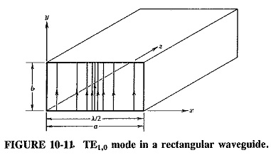
The electric field configuration is shown for the TE1,0 mode in Figure 10-11; the magnetic field is left out for the sake of simplicity but will be shown in subsequent figures. It is important to realize that the electric field extends in one direction, but changes in this field occur at right angles to that direction. This is similar to a multilane highway with graduated speed lanes. All the cars are traveling in the same direction, but with different speeds in adjoining lanes. Although all cars in any one lane travel north at high speed, along this lane no speed change is seen. However, a definite , changd in speed is noted in the east-west direction as one moves from one lane to the next. In the same way, the electric field in the TE1,0 mode extends in the y direction, but it is constant in that direction while undergoing a half-wave intensity change in the x direction. As a result, m = 1, n = 0, and the mode is thus TE1,0.
The TEm,0 modes:
Since the TEm,0 modes do not actually use the broader walls of the waveguide (the reflection takes place from the narrower walls), they are not affected by the addition of the second pair of walls. Accordingly, all the equations so far derived for the parallel-plane waveguide apply to the Rectangular Waveguide Derivation carrying TEm,0 modes, without any changes or reservations. The most important of these are Equations (10-11), (10-12), (10-15) and (10-16), of which all except the first are universal. To these equations, one other must now be added; this is the equation for the characteristic wave impedance of the waveguide. This is obviously related to Z, the characteristic impedance of free space, and is given by

where
Z0 = characteristic wave impedance of the waveguide
Although Equation (10-17) cannot be derived here, it is logically related to the other waveguide equations and to the free-space propagation conditions. It is seen that the addition of walls has increased the characteristic impedance, as compared with that of free space, for these particular modes of propagation.
It will be seen from Equation (10-17) that the characteristic wave impedance of a waveguide, for TEm,0 modes, increases as the free-space wavelength approaches the cutoff wavelength for that particular mode. This is merely the electrical analog of Equation (10-16), which states that under these conditions the group velocity decreases. It is apparent that νg = 0 and Z0 = ∞ not only occur simultaneously, when λ = λ0, but are merely two different ways of stating the same thing. The waveguide cross-sectional dimensions are now too small to allow this wave to propagate.
A glance at Equation (10-11) will serve as a reminder that the different TEm,0 modes all have different cutoff wavelengths and therefore encounter different characteristic wave impedance. Thus a given signal will encounter one value of Z0 when propagated in the TE3,0 mode, and another when propagated in the TE2,0 mode. This is the reason for the name “characteristic wave impedance.” Clearly its value depends here on the mode of propagation as well as on the guide cross-sectional dimensions.
The TEm,n modes:
The TEm,n modes are not used in practice as often as the TEm,0 modes (with the possible exception of the TE1,1 mode, which does have some practical applications). All the equations so far derived apply to them except for the equation for the cutoff wavelength, which must naturally be different, since the other two walls are also used. The cutoff wavelength for TEm,n modes is given by

Once again the derivation of this relation is too involved to go into here, but its self-consistency can be shown when it is considered that this is actually the universal cutoff wavelength equation for Rectangular Waveguide Derivation, applying equally to all modes, including the TEm,0. In the TEm,0 mode, n = 0, so that Equation (10-18) reduces to
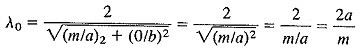
Since this is identical to Equation (10-11), it is seen that Equation (10-18) is consistent. To make calculations involving TEm,n modes, Equation (10-18) is used to calculate the cutoff wavelength, and then the same equations are used for the other calculations as were used for TEm,0 modes.
The TMm,n modes:
The obvious difference between the TMm,n modes and those described thus far is that the magnetic field here is transverse only, and the electric field has a component in the direction of propagation. This obviously will require a different antenna arrangement for receiving or setting up,such modes. Although most of the behavior of these modes is the same as for TE modes, a number of differences do exist. The first such difference is due to the fact that lines of magnetic force are closed loops. Consequently, if a magnetic field exists and is changing in the x direction, it must also exist and be changing in the y direction. Hence TMm,0 modes cannot exist (in Rectangular Waveguide Derivation). TM modes are governed by relations identical to those regulating TEm,n modes, except that the equation for characteristic wave impedance is reversed, because this impedance tends to zero when the free-space wavelength approaches the cutoff wavelength (it tended to infinity for TE modes). The situation is analogous to current and voltage feed in antennas. The formula for characteristic wave impedance for

Equation (10-19) yields impedance values that are always less than 377 Ω, and this is the main reason why TM modes are sometimes used, especially TM1.1. It is sometimes advantageous to feed a waveguide directly from a coaxial transmission line, in which case the waveguide input impedance must be a good deal lower than 377 Ω. Just as the TE1.1 is the principal TEm,n mode, so the main TM mode is the TM1.1.