Estimation of Trend Analysis in Load Forecasting:
Estimation of Trend Analysis in Load Forecasting – The simplest possible form of the deterministic part of y(k) is given by
![]()
where y̅d represents the average or the mean value of yd(k), bk represents the `trend’ term that grows linearly with k and e(k) represents the error of modelling the complete load using the average and the trend terms only. The question is one of estimating the values of the two unknown model parameters y̅d and b to ensure a good model. As seen earlier, when little or no statistical information is available regarding the error term, the method of LSE is helpful. If this method is to be used for estimating y̅d and b, the estimation index J is defined using the relation
![]()
where E(•) represents the expectation operation. Substituting for e(k) from Eq. (16.2) and making use of the first order necessary conditions for the index J to have its minimum value with respect to yd and b, it is found that the following conditions must be satisfied.
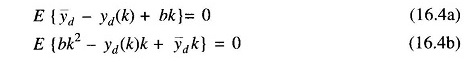
Since the expectation operation does not affect the constant quantities, it is easy to solve these two equations in order to get the desired relations.
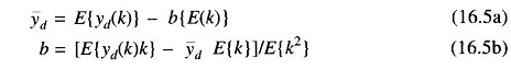
If y(k) is assumed to be stationary (statistics are not time dependent) one may involve the ergodic hypothesis and replace the expectation operation by the time averaging formula. Thus, if a total of N data are assumed to be available for determining the time averages, the two relations may be equivalently expressed as follows.
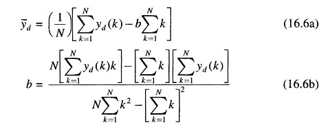
These two relations may be fruitfully employed in order to estimate the average and the trend coefficient for any given load data.
Note that Eqs. (16.6a) and (16.6b) are not very accurate in case the load data behaves as a non-stationary process since the ergodic hypothesis does not hold for such cases. It may still be possible to assume that the data over a finite window is stationary and the entire set of data may then be considered as the juxtaposition of a number of stationary blocks, each having slightly different statistics. Equations (16.6a) and (16.6b) may then be repeated over the different blocks in order to compute the average and the trend coefficient for each window of data.