Static State Estimation in Power Systems:
Static State Estimation in Power Systems – As noted earlier, for a system with N buses, the state vector x may be defined as the 2N — 1 vector of the N — 1 voltage angles δ2, …, δN and the N voltage magnitudes V1, V2, …, Vn. The load flow data, depending on type of bus, are generally corrupted by noise and the problem is that of processing an adequate set of available data in order to estimate the State Estimation vector. The readily available data may not provide enough redundancy (the large geographical area over which the system is spread often prohibits the telemetering of all the available measurements to the central computing station). The redundancy factor, defined as the ratio min should have a value in the range 1.5 to 2.8 in order that the computed value of the state may have the desired accuracy. It may be necessary to include the data for the power flows in both the directions of some of the tie lines in order to increase the redundancy factor. In fact, some `psuedo measurements’ which represent the computed values of such quantities as the active and reactive injections at some remote buses may also be included in the vector y (k).
It is thus apparent that the problem of estimation of the power system state is a non-linear problem and may be solved using either the batch processing or sequential processing formula. Also, if the system is assumed to have reached a steady-state condition, the voltage angles and magnitudes would remain more or less constant. To develop explicit solutions, it is necessary to start by noting the exact forms of the model equations for the components of the vector y (k).
Let Pi and Qi denote the active and reactive power injections of ith bus. These are related to the components of the state vector through the following equations.
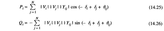
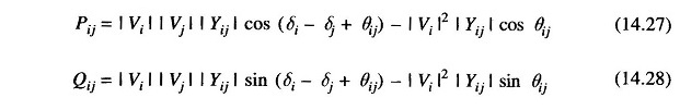
where |Yij| represents the magnitude and θij represents the angle of the admittance of the line connecting the ith and jth buses. The active and reactive components of the power flow from the ith to the jth bus, on the other hand are given by the following relations.
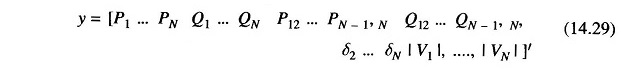
Let us assume that the vector y has the general form
The Jacobian H will then have the form
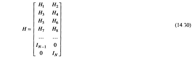
where IN is the identity matrix of dimension N, H1 is the N x (N — 1) submatrix of the partial derivatives of the active power injections wrt δ′s, H2 is the N x N sub-matrix of the partial-derivatives of the active power injections wrt |V|s is and so on. Jacobian H will also be a sparse matrix since Y is a sparse matrix.
Two special cases of interest are those corresponding to the use of only the active and reactive injections and the use of only the active and reactive line flows in the vector y. In the first case, there are a total of 2N components of y compared to the 2N — 1 components of the state x. There is thus almost no redundancy of measurements. However, this case is very close to the case of load flow analysis and therefore provides a good measure of the relative strengths of the methods of load flow and Static State Estimation. In the second case, it is possible to ensure a good enough redundancy if there are enough tie lines in the system. One can obtain two measurements using two separate meters at the two ends of a single tie-line. Since these two data should have equal magnitudes but opposite signs, this arrangement also provides with a ready check of meter malfunctioning.
The Injections Only Algorithm:
In this case, the model equation has the form
![]()
with the components of the non-linear function given by
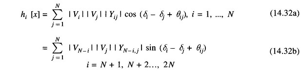
The elements of the sub-matrices H1, H2, H3 and H4 are then determined easily as follows.
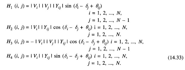
Equation (14.33) may be used to determine the Jacobian at any specified value of the system state vector. The injections only state estimation algorithm is then obtained directly. Since the problem is non-linear, it is convenient to employ the iterative algorithm given in Eq. (14.22).
![]()
Applying the principle of decoupling, the submatrices H2 and H3 become null with the result that the linearized model equation may be approximated as:

If we partition the vectors y, x and r as

then, Eq. (14.34) may be rewritten in the decoupled form as the following two separate equations for the two partitioned components of the state vector

Based on these two equations, we obtain the following nearly decoupled Static State Estimation algorithms.
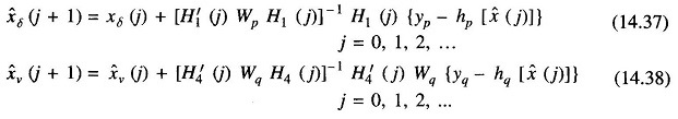
where the subscripts p and q are used to indicate the partitions of the weighting matrix W and the non-linear function h (.) which correspond to the vectors yp and yq respectively. As mentioned earlier, if the covariances Rp and Rq of the errors rp and rq are assumed known, one should select Wp= R-1p and Wq= R-1q.
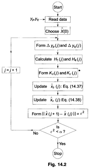
Note that Eqs. (14.37) and (14.38) are not truly decoupled because the partitions of the non-linear function depend on the estimate of the entire state vector. It may be possible to assume that νi (j) = 1 for all i and j while, Eq. (14.37) is being used in order to estimate the angle part of the state vector. Similarly one may assume δi(j) = 0° for all i and j while using Eq. (14.38) in order to estimate the voltage part of the state vector. Such approximations allow the two equations to be completely decoupled but may not yield very good solutions. A better way to decouple the two equations would be to use the load flow solutions for xν and xδ as their supposedly constant values in Eq. (14.37) and Eq. (14.38) respectively. There are several forms of fast decoupled estimation algorithms based on such considerations. A flow chart for one scheme of fast decoupled Static State Estimation in shown in Fig. 14.2.