Bad Data Detection in State Estimation of Power System:
The ability to identify Bad Data Detection in State Estimation measurements is extremely valuable to a load dispatch centre. One or more of the data may be affected by malfunctioning of either the measuring instruments or the data transmission system or,both. Transducers may have been wired incorrectly or the transducer itself may be malfunctioning so that it simply no longer gives accurate readings.
If such faulty data are included in the vector Δy, the estimation algorithm will yield unreliable estimates of the state. It is therefore important to develop techniques for detecting the presence of faulty data in the measurement vector at any given point of time, to identify the faulty data and eliminate these from the vector y before it is processed for state estimation. It is also important to modify the estimation algorithms in a way that will permit more reliable state estimation in the presence of bad data.
Bad Data Detection:
A convenient tool for detecting the presence of one or more bad data in the vector y at any given point of time is based on the ‘Chi Square Test’. To appreciate this, first note that the method of least square ensures that the performance index J(x) = [y – h (x)]’ W [y – h (x)] = r’Wr has its minimum value when x = x̂ . Since the variable r is random, the minimum value Jmin is also a random quantity. Quite often, r may be assumed to be a Gaussian variable and then Jmin would follow a chi square distribution with L = m – n degrees of freedom. It turns out that the mean of Jmin is equal to L and its variance is equal to 2L. This implies that if all the data processed for state estimation are reliable, then the computed value of Jmin should be close to the average value (=L). On the other hand, if one or more of the data for y are unreliable, then the assumptions of the least squares estimation are violated and the computed value of Jmin will deviate significantly from L.
It is thus possible to develop a reliable scheme for the Bad Data Detection in State Estimation in y by computing the value of [y – h(x̂)]′W[y – h(x̂)],x̂ being the estimate obtained on the basis of the concerned y. If the scalar so obtained exceeds some threshold Tj =cL, c being a suitable number, we conclude that the vector y includes some bad data. (Note that the data for the component yi, i = 1, 2, …, m will be considered bad if it deviates from the mean of yi by more than ±3σi, where σi is the standard deviation of ri. Care must be exercised while choosing the value of threshold parameter c. If it is close to 1, the test may produce many `false alarms’ and if it is too large, the test would fail to detect many bad data.
To select an appropriate value of c, we may start by choosing the significance level d of the test by the relation.
We may select, for example, d = 0.05 which corresponds to a 5% false alarm situation. It is then possible to find the value of c by making use of the table X(L). Once the value of c is determined, it is simple to carry out the test whether or not J (x) exceeds cL.
Identification of Bad Data:
Once the presence of bad data is detected, it is imperative that these be identified so that they could be removed from the vector of measurements before it is processed. One way of doing this is to evaluate the components of the measurement residual ÿi = yi – hi (x), i=1, 2,…m. If we assume that the residuals have the Gaussian distribution with zero mean and the variance σ2i, then the magnitude of the residual yi should lie in the range -3σi < yi <3σi with 95% confidence level. Thus, if any one of the computed residual turns out to be significantly larger in magnitude than three times its standard deviation, then corresponding data is taken to be a bad data. If this happens for more than one component of y, then the component having the largest residual is assumed to be the bad data and is removed from y. The estimation algorithm is re-run with the remaining data and the Bad Data Detection in State Estimation and identification tests are performed again to find out if there are additional bad data in the measurement set. As we will see later bad measurement data are detected, eliminated and replaced by pseudo or calculated values.
Suppression of Bad Data:
The procedures described so far in this section are quite tedious and time consuming and may not be utilized to remove all the bad data which may be present in the vector y at a given point of time. It may often be desirable on the other hand to modify the estimation algorithms in a way that will minimise the influence of the bad data on the estimates of the state vector. This would be possible if the estimation index J(x) is chosen to be a non-quadratic function. The reason that the LSE algorithm does not perform very well in the presence of bad data is the fact that because of the quadratic nature of J(x), the index assumes a large value for a data that is too far removed from its expected value. To avoid this overemphasis on the erroneous data and at the same time to retain the analytical tractability of the quadratic performance index, let us choose
![]()
where g (ÿ) is a non-linear function of the residual ÿ . There may be several possible choices for this function. A convenient form is the so-called ‘quadratic flat’ form. In this case, the components of the function g (y) are defined by the following relation.
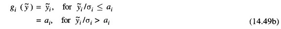
where ai is a pre-selected constant threshold level. Obviously, the performance index J(x) may be expressed as
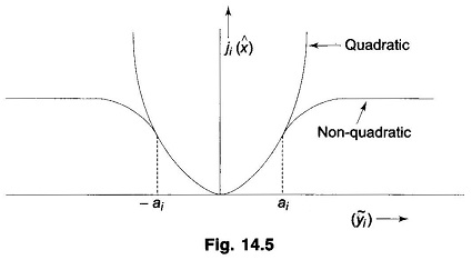
and each component has a quadratic nature for small values of the residual but has a constant magnitude for residual magnitudes in excess of the threshold. Figure 14.5 shows a typical variation of Ji (x) for the quadratic and the non-quadratic choices.
The main advantage of the choice of the form (14.49) for the estimation index is that it is still a quadratic in the function g (ÿ) and so the LSE theory may be mimicked in order to derive the following iterative formula for the state estimate.
![]()
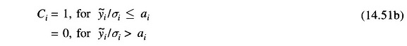
where the matrix C is diagonal and its elements are computed as
![]()
Comparing this solution with that given in Eq. (14.22), it is seen that the main effect of the particular choice of the estimation index in Eq. (14.49) is to ensure that the data producing residuals in excess of the threshold level will not change the estimate. This is achieved by the production of a null value for the matrix C for large values of the residual.