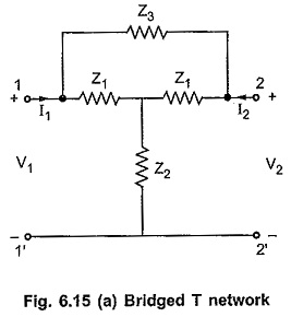
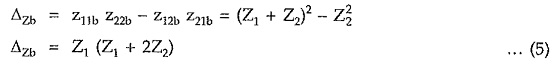
Bridged T Network Analysis:
Consider Bridged T Network Analysis as shown in the Fig. 6.15 (a).
We can consider bridged T network as a parallel connection of the two networks as shown in the Fig. 6.15 (b). The y-parameters of the overall network can be obtained by adding y-parameters of networks connected in parallel.
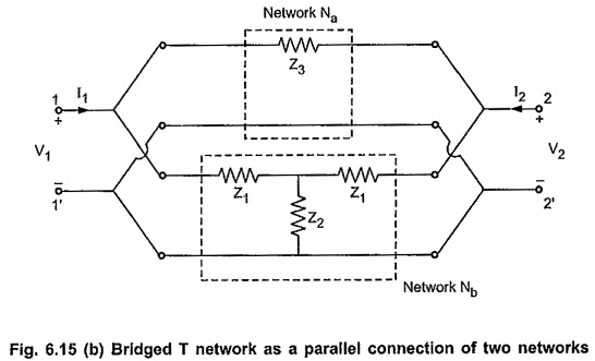
The parameters of the network Na are given by
Consider the network Nb. As the network is symmetrical T network, we can write Z-parameters of the network directly as follows,
From equations (3) and (4),
Hence y-parameters of the network Nb are given by
As both the networks Na and Nb are symmetrical so the overall bridged T network is also symmetrical network. Hence overall y-parameters for the bridged T network are obtained by adding y-parameters of the networks Na and Nb.
Ladder Network:
The Fig. 6.16 shows a ladder network. The Z1,Z3, ….Zn-1 are the impedances in series arms while Y2,Y4 …..Yn are the admittances in shunt arms.
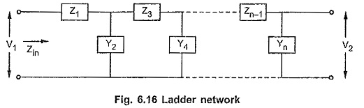
The Zin is the input impedance function of the ladder network.
Analysis of Ladder Network [Unit Output Method]:
The continued fraction method of finding driving point impedance of the network is already discussed. Let us study another simple method of obtaining network functions of a ladder network.
This method is based only on the relationships that exist between the branch currents and the node voltages of the ladder. In this method we name the various node voltages and branch currents and start at the output end, analyzing the network back to the input end.
Consider a four branch ladder network as shown in the Fig. 6.17, to understand the method.
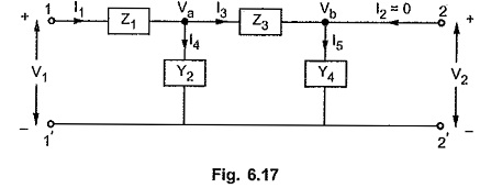
The various node voltages and branch currents are indicated. Analyse the output end.
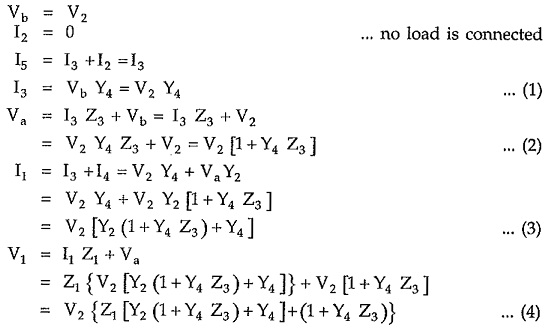
It can be observed that each equation depends on the earlier two equations only. Each new equation takes into account one new immitance (either impedance or admittance). The each new equation is obtained by multiplying the equation just preceding it by the immitance that is next down the line and then adding to this product, an equation which is twice preceding it.
For example consider equation (2). The next equation is obtained by multiplying this equation by Y2 which is next admittance down the line and adding to it an equation (1) which is twice preceding the new equation.
Thus general procedure for the analysis is,
- Write alternately the node voltage and branch current equations.
- The next equation is obtained by multiplying the existing equation by the next immitance, analyzing from port 2 to 1 i.e. from right to left and adding to this the result of the previous equation.
Using these equations any network function such as driving point imittance, voltage ratio transfer function and current ratio transfer function can be obtained.
The method discussed above is called unit output method as every equation contain V2 factor which can be normalized to V2 = 1.