Symmetrical Optimum:
Symmetrical Optimum – Sometimes automatic control systems contain integrating also besides first order delay elements, proportional elements and deadzones. Such a system when compensated on the basis of magnitude optimum discussed in the previous sections will become oscillatory with zero damping. As has already been explained the magnitude optimum utilizes a PI controller to compensate the effects of largest time constant of the system. The other first order delays present are replaced by a single delay which is the sum of all the other uncompensated delays. The rise time of the system decreases. The amplification of the proportional element is
![]()
If this principle is employed to compensate the system with integrating element, the integrating element of the compensator combines with that of the system resulting in a double integration. The characteristic equation of the closed loop system contains only s2 and constant terms showing that the system has no damping. The system has sustained oscillations. This can be illustrated by considering a system having an integrator and a first order delay in cascade.
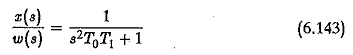
The open loop transfer function of the system is
![]()
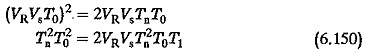
Using the principle of magnitude optimum Tn = T1. Therefore,
![]()
The closed loop transfer function is
![]()
assuming VRVs = 1 (as a special case). The term containing s is not present in the characteristic equation which clearly shows that the damping is zero. Also we know that
The differential equation representing the system is
![]()
For a step input the response of the system is given by
![]()
is representative of sustained oscillations.
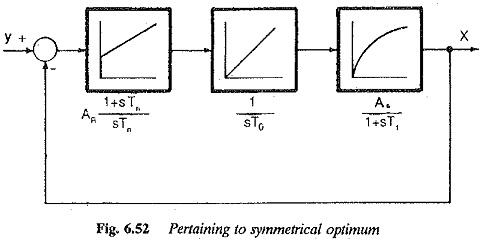
Therefore the controller design to compensate the effect of the dominant poles of the system is based on the principle of symmetrical optimum. The frequency response of the compensated system is symmetrical about gain cross over frequency.
The criteria for this optimum are derived in the following. The system contains an integration time of T0 and a first order delay of T1 (Fig. 6.52). A PI controller is used to compensate the system. In magnitude optimum the criteria have been developed assuming that the amplitude of transfer function is unity in the complete range of frequencies. In the present case, the criteria for symmetrical optimum are developed so that the transfer function has an amplitude of unity over a restricted range of frequencies.
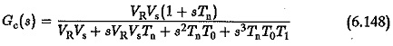
The open loop transfer function of the compensated system
![]()
The closed loop transfer function is
The amplitude of frequency response
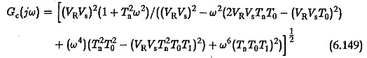
The system has apparently a damped response as the characteristic equation has all powers of present and the coefficients are positive. The amplitude is unity at zero frequency. However, it approaches unity in a certain frequency range if the following conditions are satisfied.
These lead to a result that the reset time of the integrator.
![]()
and the proportional amplification is
![]()
The integration time constant will always include the amplification of the integrator also. Therefore T0/Vs can be considered as Ti, the integration time.
Thus,![]()
The closed loop transfer function of the system is
![]()
This is the general form of the transfer function of the compensated system based on symmetrical optimum. The amplitude plot of the open loop transfer function of the compensated system is shown in Fig. 6.53. The plot shows a symmetry about the corner frequencies 1/4T1 and 1/T1 with respect to gain cross over frequency 1/2T1 on the 0 — dB axis. This property justifies the name symmetrical optimum.
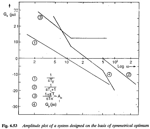
The system compensated by this principle has its behaviour decided by the time constant T1 (the sum of all parasitic time constants).
The time response of the system is given by solving the differential equation
![]()
For a step input the time response of the system is given by
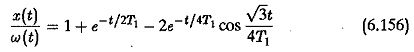
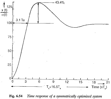
and it is shown in Fig. 6.54. It has a rise time of 3.1 T1, a peak overshoot of 43.4%, and a settling time of 16.5T1.
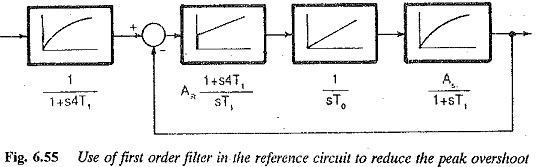
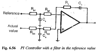
This large overshoot of the system is due to the factor 1 + s4T1 in the numerator. If the reference input to the controller is delayed by a first order delay of transfer function 1/(s4T1+1), the overshoot can be reduced to 8%. This is shown in Fig. 6.55. The rise time in this case increases to 7.6T1. The PI controller with delay in the reference input is shown in Fig. 6.56.
If the system contains delay elements such that the largest time constant is greater than the four times the sum of all other small time constants this method can be employed for compensation. If T1,T2,T3,T4,… are time constants of the system such that
![]()
the first order delay with time constant T1 can be considered an integration in the system compared to the other time constants.