Magnitude Optimum:
The design of a controller based on the principle Magnitude Optimum that it allows all the frequencies to pass through in a similar way for a simple system is shown in Fig. 6.31.
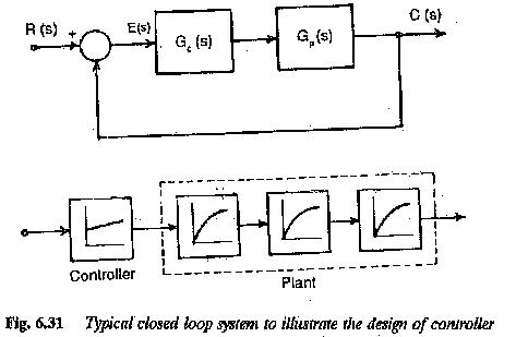
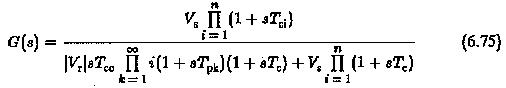
The system has an input R(s) and output C(s). The closed loop transfer function
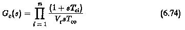
The plant transfer function Gp(s) is assumed to be having linear factors and is given by
Where
Vs is the gain of the plant
TPK large time constants of the system
Te sum of all parasitic time constants.
These parasitic time constants of the control system are introduced by the non-ideal nature of the devices and the elements used for harmonic elimination and smoothing. The value of Te is of the order of 2 to 5 ms and it is very much smaller than the least of the large time constants.
The controller designed is a PID controller which has a general transfer function given by
Using Eqs 6.73 and 6.74 in Eq. 6.72 we have the overall closed loop function given by
An optimised controller can be obtained on the principle described only if the large time constants are compensated and T0 and Te only effect the transient behaviour. Hence the rules of optimization can be stated as
- the number of large time constants in the numerator and the denominator must be the same.
- the values of time constants must be the same.
- The time constant of integration of controller must be fixed as T0 = (Vs/Vr)2Te.
For a specific case of a second order system having a transfer function G
![]()
the controller must have a transfer function
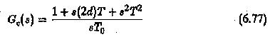
Using the above rules of optimization
![]()
If the controller suits the plant with respect to its structure as well as parameters, typical transfer functions are given both for open and closed loops.
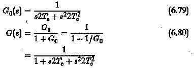
This can be obtained directly from the transfer function by applying the criterion that the overall transfer function should have a magnitude which is the same for all ω.
The plant transfer function is
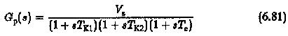
The controller transfer function is
![]()
The open loop transfer function is
![]()
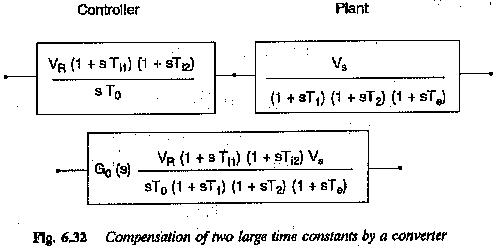
Making Ti1 = T1,Ti2 = T2 so that controller completely compensates both the large time constants of the plant we have
![]()
The closed loop transfer function
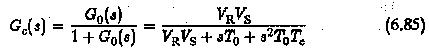
Its frequency response
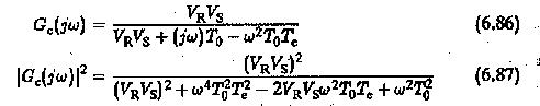
must be unity to satisfy the magnitude optimum. This happens only if
![]()
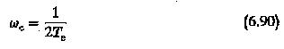
The compensation of the two large time constants of the plant by the controller is depicted in Fig. 6.32. The Bode plot of the open loop transfer function corresponds to a first order system with integration. The gain cross-over frequency
The phase margin at gain cross-over is 65°.
The time response of the modified system with the controller can now be determined. The closed loop transfer function
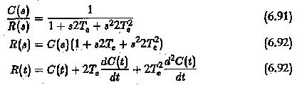
Assuming zero initial conditions, i.e.,
![]()
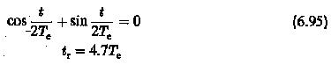
We have the time response (Fig. 6.33)
![]()
1.The rise time tr is the time taken by the output to attain the input value for the first time
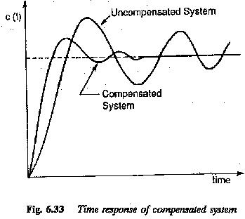
2.The settling time is determined using the fact that it takes several cycles for the output quantity to reach the steady-state value
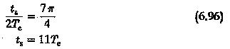
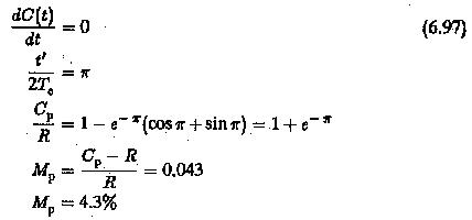
3.The overshoot is determined using the condition
The resulting system will have a damping factor 0.707 as decided by the ratio of time constants. This damping is rather high and may not be suitable for all applications.