Optimum Generation Scheduling:

Optimum Generation Scheduling – From the unit commitment table of a given plant, the fuel cost curve of the plant can be determined in the form of a polynomial of suitable degree by the method of least squares fit. If the transmission losses are neglected, the total system load can be optimally divided among the various generating plants using the equal incremental cost criterion. It is, however, unrealistic to neglect transmission losses particularly when long distance transmission of power is involved.

A modern electric utility serves over a vast area of relatively low load density. The transmission losses may vary from 5 to 15% of the total load, and therefore, it is essential to account for losses while developing an economic load dispatch policy. It is obvious that when losses are present, we can no longer use the simple ‘equal incremental cost’ criterion. To illustrate the point, consider a two-bus system with identical generators at each bus (i.e. the same IC curves). Assume that the load is located near plant 1 and plant 2 has to deliver power via a lossy line. Equal incremental cost criterion would dictate that each plant should carry half the total load; while it is obvious in this case that the plant 1 should carry a greater share of the load demand thereby reducing transmission losses.

In this section, we shall investigate how the load should be shared among various plants, when line losses are accounted for. The objective is to minimize the overall cost of generation

at any time under equality constraint of meeting the load demand with transmission loss, i.e.

Where

• k = total number of generating plants
• P_Gi = generation of ith plant
• P_D = sum of load demand at all buses (system load demand)
• P_L = total system transmission loss

To solve the problem, we write the Lagrangian as

It will be shown later in this section that, if the power factor of load at each bus is assumed to remain constant, the system loss P_L can be shown to be a function of active power generation at each plant, i.e.

 

Thus in the optimization problem posed above, P_Gi (i = 1, 2, …, k) are the only control variables.

For Optimum Generation Scheduling real power dispatch,

Rearranging Eq. (7.22) and recognizing that changing the output of only one plant can affect the cost at only that plant, we have

where

is called the penalty factor of the ith plant.

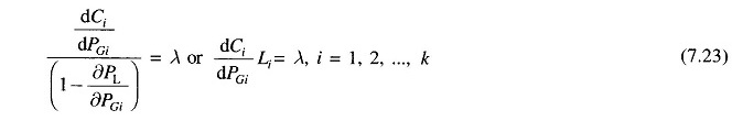
The Lagrangian multiplier λ is in rupees per megawatt-hour, when fuel cost is in rupees per hour. Equation (7.23) implies that minimum fuel cost is obtained, when the incremental fuel cost of each plant multiplied by its penalty factor is the same for all the plants.

The (k + 1) variables (P_G1, P_G1,… P_GK, λ) can be obtained from k optimal dispatch Eq. (7.23) together with the power balance Eq. (7.19). The partial derivative δP_L/δP_Gi is referred to as the incremental transmission loss (ITL)_i, associated with the ith generating plant.

Equation (7.23) can also be written in the alternative form

This equation is referred to as the exact coordination equation.

Thus it is clear that to solve the Optimum Generation Scheduling problem, it is necessary to compute ITL for each plant, and therefore we must determine the functional dependence of transmission loss on real powers of generating plants. There are several methods, approximate and exact, for developing a transmis­sion loss model. A full treatment of these is beyond the scope of this book. One of the most important, simple but approximate, methods of expressing transmission loss as a function of generator powers is through B-coefficients. This method is reasonably adequate for treatment of loss coordination in economic scheduling of load between plants. The general form of the loss formula (derived later in this section) using B-coefficients is

If P_Gs are in megawatts, B_mn are in reciprocal of megawatts. Computations, of course, may be carried out in per unit. Also, B_mn = B_nm.

Equation (7.26) for transmission loss may be written in the matrix form as

Where

It may be noted that B is a symmetric matrix.

For a three plant system, we can write the expression for loss as

With the system power loss model as per Eq. (7.26), we can now write

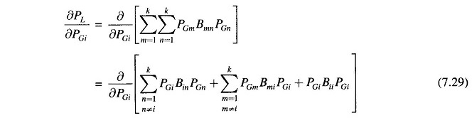
It may be noted that in the above expression other terms are independent of P_Gi and are, therefore, left out.

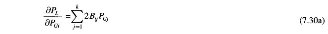
Simplifying Eq. (7.29) and recognizing that B_ij = B_ji, we can write

Assuming quadratic plant cost curves as

We obtain the incremental cost as

Substituting δP_L/δP_Gi and dC_i/dP_Gi from above in the coordination Eq. (7.22), we have

Collecting all terms of P_Gi and solving for P_Gi, we obtain

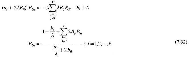
For any particular value of λ, Eq. (7.32) can be solved iteratively by assuming initial values of P_Gis(a convenient choice is P_Gi = 0; i = 1, 2, …, k). Iterations are stopped when P_Gis converge within specified accuracy.

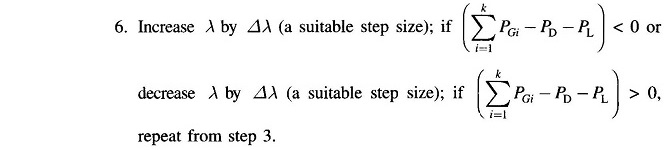
Equation (7.32) along with the power balance Eq. (7.19) for a particular load demand P_D are solved iteratively on the following lines:

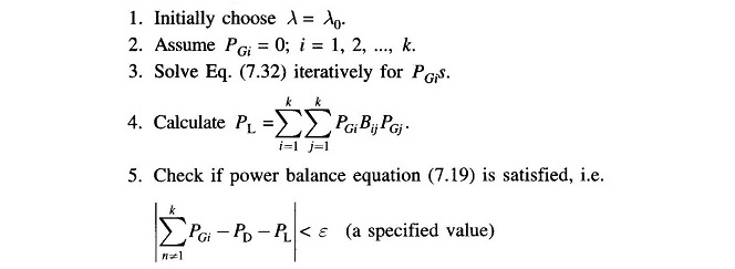
If yes, stop. Otherwise go to step 6.