Derivation of Transmission Loss Formula:
An accurate method of obtaining a general derivation of transmission loss formula has been given by Kron. This, however, is quite complicated. The aim of this article is to give a simpler derivation by making certain assumptions.
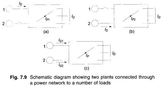
Figure 7.9 (c) depicts the case of two generating plants connected to an arbitrary number of loads through a transmission network. One line within the network is designated as branch p.
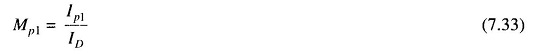
Imagine that the total load current ID is supplied by plant 1 only, as in Fig. 7.9a. Let the current in line p be IP1. Define
Similarly, with plant 2 alone supplying the total load current (Fig. 7.9b), we can define
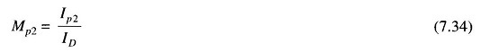
MP1 and MP2 are called current distribution factors. The values of current distribution factors depend upon the impedances of the lines and their interconnection and are independent of the current ID.
When both generators 1 and 2 are supplying current into the network as in Fig. 7.9(c), applying the principle of superposition the current in the line p can be expressed as
![]()
where IG1 and IG2 are the currents supplied by plants 1 and 2, respectively.
At this stage let us make certain simplifying assumptions outlined below:
1. All load currents have the same phase angle with respect to a common To understand the implication of this assumption consider the load current at the ith bus. It can be written as
![]()
where δi is the phase angle of the bus voltage and Φi is the lagging phase angle of the load. Since δi and Φi vary only through a narrow range at various buses, it is reasonable to assume that θi is the same for all load currents at all times.
2. Ratio X/R is the same for all network branches.
These two assumptions lead us to the conclusion that IP1 and ID [Fig. 7.9(a)] have the same phase angle and so have IP2 and ID [Fig. 7.9(b)], such that the current distribution factors MP1 and MP2 are real rather than complex.
Let,
![]()
where σ1 and σ2 are phase angles of IG1 and IG2, respectively with respect to the common reference.
From Eq. (7.35), we can write
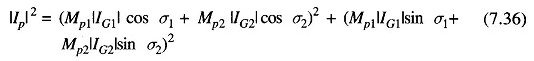
Expanding the simplifying the above equation, we get
![]()
Now
![]()
where PG1 and PG2 are the three-phase real power outputs of plants 1 and 2 at power factors of cos Φ1, and cos Φ2, and V1 and V2 are the bus voltages at the plants.
If RP is the resistance of branch p, the total derivation of transmission loss formula is given by
![]()
Substituting for |IP|2 from Eq. (7.37), and |IG1| and |IG2| from Eq. (7.38), we obtain
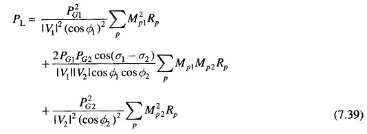
Equation (7.39) can be recognized as
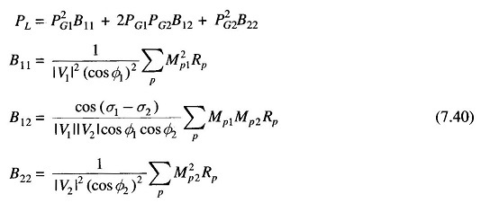
The terms B11, B12 and B22 are called loss coefficients or B-coefficients. If voltages are line to line kV with resistances in ohms, the units of B-coefficients are in MW-1. Further, with PG1 and PG2 expressed in MW, PL will also be in MW.
The above results can be extended to the general case of k plants with transmission loss expressed as
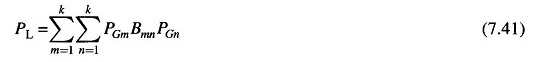
Where
![]()
The following assumptions including those mentioned already are necessary, if B-coefficients are to be treated as constants as total load and load sharing between plants vary. These assumptions are:
- All load currents maintain a constant ratio to the total current.
- Voltage magnitudes at all plants remain constant.
- Ratio of reactive to real power, i.e. power factor at each plant remains
- Voltage phase angles at plant buses remain fixed. This is equivalent to assuming that the plant currents maintain constant phase angle with respect to the common reference, since source power factors are assumed constant as per assumption 3 above.
In spite of the number of assumptions made, it is fortunate that treating B-coefficients as constants, yields reasonably accurate results, when the coefficients are calculated for some average operating conditions. Major system changes require recalculation of the coefficients.
Losses as a function of plant outputs can be expressed by other methods, but the simplicity of loss equations is the chief advantage of the B-coefficients method.
Accounting for derivation of transmission loss formula results in considerable operating economy. Furthermore, this consideration is equally important in future system planning and, in particular, with regard to the location of plants and building of new transmission lines: