Salient Pole Synchronous Generator:

A Salient Pole Synchronous Generator, as shown in Fig. 4.29, is distinguished from a round rotor machine by constructional features of field poles which project with a large interpolar air gap. This type of construction is commonly employed in machines coupled to hydroelectric turbines which are inherently slow-speed ones so that the Salient Pole Synchronous Generator has multiple pole pairs as different from machines coupled to high-speed steam turbines (3,000/1,500 rpm) which have a two- or four-pole structure. Salient Pole Synchronous Generator analysis is made through the two-reaction theory outlined below.

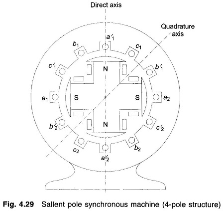
In a round rotor machine, armature current in phase with field induced emf E_f or in quadrature (at 90°) to E_f produces the same flux linkages per ampere as the air gap is uniform so that the armature reaction reactance offered to in-phase or quadrature current is the same (X_a + X_l = X_s). In a salient pole machine air gap is non-uniform along rotor periphery. It is the least along the axis of main poles (called direct axis) and is the largest along the axis of the interpolar region (called quadrature axis). Armature current in quadrature with E_f  produces flux along the direct axis and the reluctance of flux path being low (because of small air gap), it produces larger flux linkages per ampere and hence the machine presents larger armature reaction reactance X_d (called direct axis reactance) to the flow of quadrature component I_d of armature current I_a. On the other hand, armature current in phase with E_f produces flux along the quadrature axis and the reluctance of the flux path being high (because of large interpolar air gap), it produces smaller flux linkages per ampere and hence the machine presents smaller armature reaction reactance X_q (quadrature axis reactance < X_d) to the flow of inphase component I_q of armature current I_a.

Since a salient pole machine offers different reactances to the flow of I_d and l_q components of armature current I_a, a circuit model cannot be drawn.

Phasor Diagram of Salient Pole Synchronous Machine:

The Phasor Diagram of Salient Pole Synchronous generator is shown in Fig. 4.30. It can be easily drawn by following the steps given below:

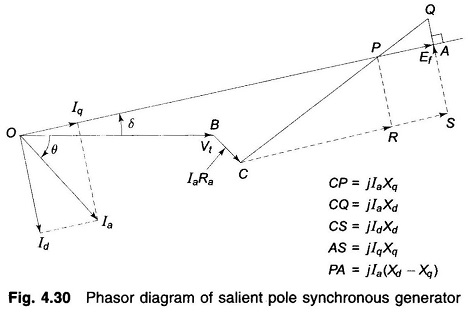
1. Draw V_t and I_a at angle θ
2. Draw I_aR_a. Draw CQ = jl_aX_d(⊥ to I_a)
3. Make |CP| = |I_a|X_q and draw the line OP which gives the direction of E_f phasor
4. Draw a ⊥ from Q to the extended line OP such that OA = E_f

It can be shown by the above theory that the power output of a salient pole generator is given by

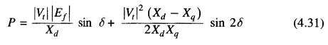
The first term is the same as for a round rotor machine with X_s = X_d and constitutes the major part in power transfer. The second term is quite small (about 10-20%) compared to the first term and is known as reluctance power.

Power Angle Curve for Salient Pole Synchronous Machine:

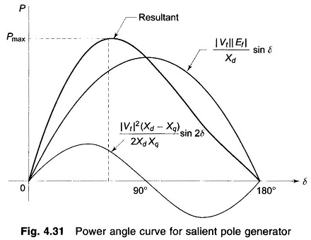
P versus δ is plotted in Fig. 4.31. It is noticed that the maximum power output occurs at δ < 90° (about 70°). Further dp/dδ (change in power per unit change in power angle for small changes in power angle), called the synchronizing power coefficient, in the operating region (δ < 70°) is larger in a salient pole machine than in a round rotor machine.

Here, we shall neglect the effect of saliency and take

in all types of power system studies considered.

During a machine transient, the direct axis reactance changes with time acquiring the following distinct values during the complete transient.

• X″_d = subtransient direct axis reactance
• X′_d = transient direct axis reactance
• X_d = steady state direct axis reactance

Operating Chart of Synchronous Generator:

While selecting a large generator, besides rated MVA and power factor, the greatest allowable stator and rotor currents must also be considered as they influence mechanical stresses and temperature rise. Such limiting parameters in the operation are brought out by means of an operating chart or performance chart.

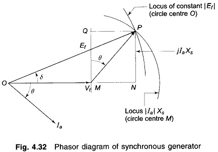
For simplicity of analysis, the saturation effects, saliency, and resistance are ignored and an unsaturated value of synchronous reactance is considered. Consider Fig. 4.32, the phasor diagram of a cylindrical rotor machine. The locus of constant |I_a|X_s,|I_a| and hence MVA is a circle centered at M. The locus of constant |E_f| (excitation) is also a circle centered at O. As MP is proportional to MVA, QP is proportional to MVAR and MQ to MW, all to the same scale which is obtained as follows.

For zero excitation,

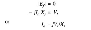
i.e. |I_a|=|V_t|/X_s leading at 90° to OM which corresponds to VARs/phase.

Consider now the chart shown in Fig. 4.33 which is drawn for a synchronous machine having X₃ = 1.43 pu. For zero excitation, the current is 1.0/1.43 = 0.7 pu, so that the length MO corresponds to reactive power of 0.7 pu, fixing both active and reactive power scales.

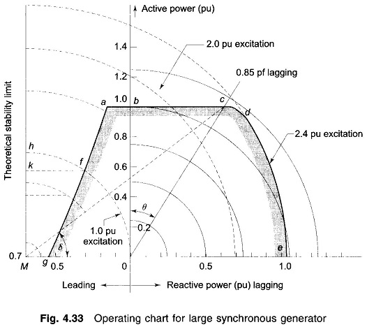
With centre at 0 a number of semicircles are drawn with radii equal to different pu MVA loadings. Circles of per unit excitation are drawn from centre M with 1.0 pu excitation corresponding to the fixed terminal voltage OM. Lines may also be drawn from 0 corresponding to various power factors but for clarity only 0.85 pf lagging line is shown. The operational limits are fixed as follows.

Taking 1.0 per unit active power as the maximum allowable power, a horizontal limit-line abc is drawn through b at 1.0 pu. It is assumed that the machine is rated to give 1.0 per unit active power at power factor 0.85 lagging and this fixes point c. Limitation of the stator current to the corresponding value requires the limit-line to become a circular arc cd about centre 0. At point d the rotor heating becomes more important and the arc de is fixed by the maximum excitation current allowable, in this case assumed to be |E_f| = 2.40 pu (i.e. 2.4 times |V_t|. The remaining limit is decided by loss of synchronism at leading power factors. The theoretical limit is the line perpendicular to MO at M (i.e. δ = 90°), but in practice a safety margin is brought in to permit a further small increase in load before instability. In Fig. 4.33, a 0.1 pu margin is employed and is shown by the curve afg which is drawn in the following way.

Consider a point h on the theoretical limit on the |E_f| = 1.0 pu excitation arc, the power Mh is reduced by 0.1 pu to Mk; the operating point must, however, still be on the same |E_f| arc and k is projected to f which is the required point on the desired limiting curve. This is repeated for other excitations giving the curve afg. The complete working area, shown shaded, is gfabcde. A working point placed within this area at once defines the MVA, MW, MVAR, current, power factor and excitation. The load angle δ can be measured as shown in the figure.