Pole Zero Plot:
Pole Zero Plot – The variable s is a complex variable. Hence a complex plane is required to indicate the values of s graphically. A complex plane is a plane with X-axis as real axis and Y-axis as imaginary axis. The real axis is denoted as σ axis while imaginary axis is denoted as jω axis. Such a complex plane used to indicate values of s in it is called s-plane. All the poles and zeros can be easily indicated in such a s-plane.
The poles are indicated by symbol ‘cross’ (X), in s-plane.
The zeros are indicated by symbol of ‘small circle’ (O) in s-plane.
The plot obtained by locating all the poles and zeros of the network function in s-plane is called Pole zero plot of that network function.
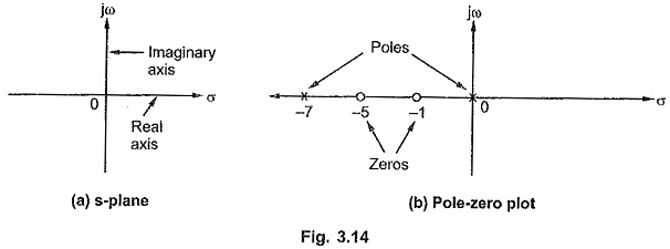
The s-plane is shown in the Fig. 3.14 (a).
While consider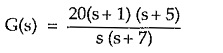
whose pole-zero plot is shown in the Fig. 3.14 (b).
The scale factor of a network function can not be indicated on the pole-zero plot. Thus while obtaining network function from the pole-zero plot, additional information is necessary to obtain the scale factor of a network function. For the repeated poles or zeros, the marks equal to the number of repeated poles or zeros must be shown in the pole-zero plot.
Significance of Poles and Zeros:
The network function is always the ratio of Laplace of the output to the input. Thus if the input is known, it is easy to obtain the expression for the Laplace transform of the output variable, from the network function.
Thus if,
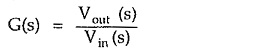
Then,
![]()
Now to find the response in the time domain, it is necessary to find inverse Laplace transform of Vout(s), which is possible by expanding it in partial fraction expansion form.
It is important to note that the partial fraction expansion depends on the denominator of the Laplace transform of the output variable i.e. the poles of the output function.
If F(s) in the output variable then for each real pole of F(s), there exists an exponential term in the time domain.
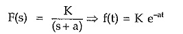
For a quadratic pole with purely imaginary roots, as the poles of F(s), there exists sine or cosine term in the time domain.
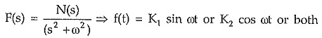
similarly a quadratic with complex conjugate roots as the poles of F(s) produce damped sine or damped cosine type of terms in the time domain.
While the partial fraction coefficients are decided by the zeros of the function F(s).
Thus the poles determine the waveform of the time variation of the response while the zeros determine the magnitude of each part of the response.
We have seen that driving point functions can be the impedance Z(s) functions or admittance Y(s) functions. Hence these are called immitance functions.
If driving point function is an impedance function i.e.
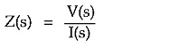
Then zero of Z(s) means zero voltage for a finite current i.e. short circuit condition in practice.
While a pole of Z(s) means zero current for a finite voltage i.e. open circuit condition in practice.
Hence for poles, a one terminal pair network acts as an open circuit while for zeros it acts as short circuit. As the poles and zeros are critical frequencies, practically poles and zeros indicate the frequencies for which the network acts as an open circuit or short circuit. To understand this, consider transform impedance of single capacitor as Z(s) = 1/sC. It has a pole at s = 0 thus for a zero frequency i.e. at s = 0, Z(s) = ∞ i.e. it acts as an open circuit. While this Z(s) has a zero value for s = ∞ i.e. a zero at s = ∞ for which it acts as short circuit.