Time Domain Response From Pole Zero Plot:

From the locations of poles and zeros of the network function in the s-plane, the time response of the network can be perfectly identified. Let us study the various types of poles and their locations and the related time Time Domain Response From Pole Zero Plot. As stated earlier, poles mainly decide the nature of the response while the zeros decide the magnitude of each part of the response.

Case 1 : Real and negative pole

Consider the network function with real and negative pole located at s = – a.

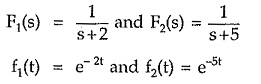
The location of pole and corresponding Time Domain Response From Pole Zero Plot is shown in the Fig. 3.17 (a) and (b).

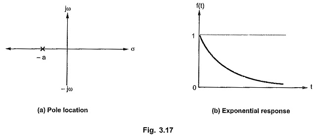
Thus a real negative pole always produces an exponentially decaying time response.

Consider

The pole-zero plot and responses are shown in the Fig. 3.18 (a) and (b).

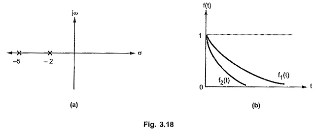
It can be seen that as pole moves away from origin, on the real axis, in the left half of s-plane, the corresponding time response exponentially decays at a faster rate.

Case 2 : Real, negative, repetitive pole

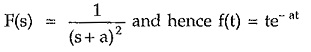
Consider a function with presence of double order pole at s = – a.

The location of poles and corresponding time response is shown in the Fig. 3.19 (a) and (b).

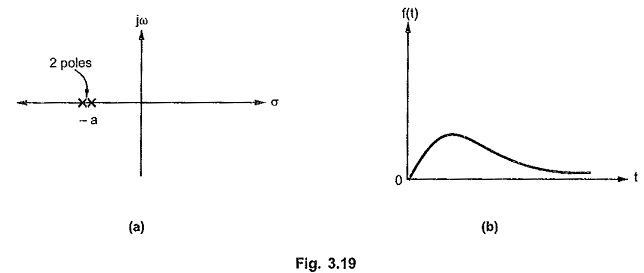
The double power produces ‘t’ in the time response but as it is associated with exponential term of negative power due to negative real part of pole, the response is going to vanish as t -> ∞ starting from origin.

But if the real part of such pole is made zero i.e. double pole is shifted at origin, then corresponding time response looses the exponential negative power term, giving ramp type of response which increases to so as t -> ∞. Such networks are said to be unstable in nature.

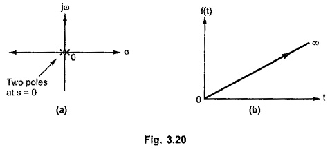
So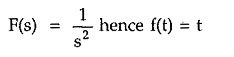

Thus double poles at origin is not preferred in the network function which produces unstable response in practice.

Case 3 : Real, positive pole

Consider a network function with a pole at s = + a.

The location of pole and corresponding time response is shown in the Fig. 3.21 (a) and (b).

It can be observed that any pole with positive real part of any order, produces an exponential term of positive index in the corresponding Time Domain Response From Pole Zero Plot. But as t -> ∞, such term produces uncontrollable time response which also tends to ∞. Hence in practice, for a stable, controllable network function there should not be a single pole with positive real part. Thus for stability of the network, no pole should be located in the right half of s-plane.

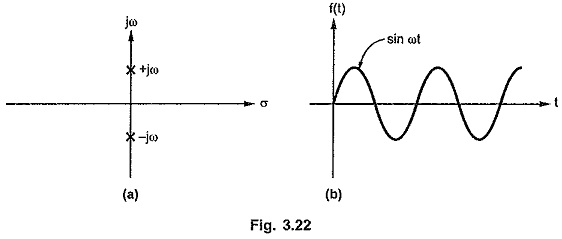
Case 4 : Complex poles on imaginary axis.

Consider a network function with complex poles located on imaginary axis.

The poles are located at s = ± j ω from s² + ω² = 0.

The locations of poles and corresponding time response is shown in the Fig. 3.22 (a) and (b).

If such a pair of poles has a zero at origin or a finite zero then in the corresponding time response, cosine waveform or both sine and cosine waveforms are present.

If

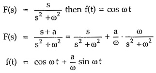
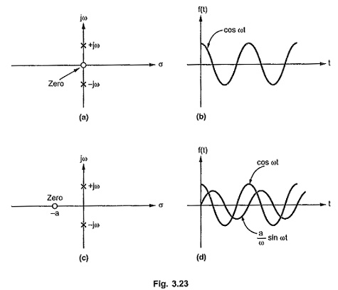
But it can be observed that the frequency of the sine and cosine terms in f(t) is decided by the magnitude of the poles located on the imaginary axis.

It can also be observed that as the pair of complex poles (±jω) moves away from the origin, the frequency of the sinusoidal terms in the time response is more and viceversa. Thus purely imaginary complex poles produce purely sinusoidal terms in the Time Domain Response From Pole Zero Plot.

Case 5 : Complex poles with negative real part.

Consider a network function with a quadratic factor as its poles having complex conjugate roots with negative real part.

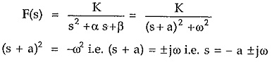
Completing square it can be adjusted in the standard form as (s + a)² + ω².

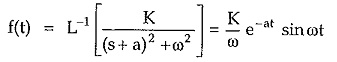
It can be seen that the negative real part of the roots appears as exponential term with negative power while complex nature of poles produce sinusoidal terms in the time response. So the corresponding time domain response is damped oscillations i.e. oscillations with decreasing amplitude. The pole-zero plot and the corresponding time response is shown in the Fig. 3.24 (a) and (b)

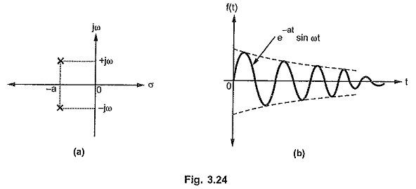
Each such pair of complex conjugate poles with negative real part produces damped oscillatory time response. The frequency of such oscillatory terms depends on the imaginary part of the complex conjugate poles producing them. If there is a zero, along with such complex conjugate pair of poles in the network function then there exists both e^-at sin ωt and e^-at cos ωt in the corresponding time response.

Case 6 : Complex poles with positive real part

Consider a network function with a pair of complex conjugate poles with positive real part. Then the positive real part of poles produces exponential term with positive index along with the oscillatory term, in the corresponding time response.

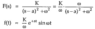
As t → ∞, the amplitude of such oscillations increases towards ∞. Such oscillations are called growing oscillations.

The pole-zero plot and the corresponding time response for such case is shown in the Fig. 3.25 (a) and (b).

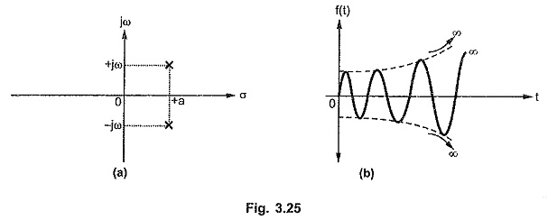
Such a time response is uncontrollable and such a network is said to be unstable in nature.

Case 7 : Repeated pair of poles on the imaginary axis.

Consider a network function with repeated pair of poles on the imaginary axis.

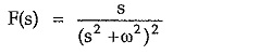
The corresponding time response is,

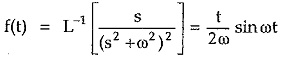
The repetitive nature of poles produces function t along with sin ωt. Thus as t → ∞, the response also approaches to ∞. So such oscillations are oscillations with increasing amplitude. This indicates unstable nature of the network.

The pole-zero plot and the corresponding time response is shown in the Fig. 3.26 (a) and (b).

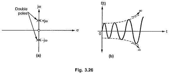
Thus the multiple poles on the imaginary axis are responsible for the unstable network response.

Case 8 : Single pole at the origin.

Consider a network function with single pole at the origin.

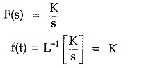
Thus it is a step type of time response corresponding to the pole at the origin.

The pole location and the corresponding time response is shown in the Fig. 3.27 (a) and

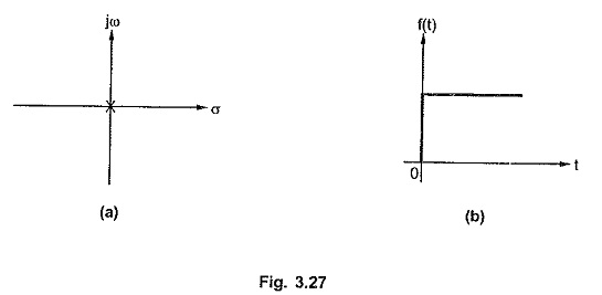
Thus a pole at the origin represents a step type time function but the magnitude of the step K must be identified from the s-domain network function as constant K can not be indicated on the pole-zero plot.

Thus a nature of the time response f(t) can be predicted from the pole-zero plot of the network function. From the discussion of the above cases it can be concluded that locations of poles in the left half of s-plane, whether real or complex, are responsible for stable, controllable response. While the poles located in the right half of s-plane are responsible for the unstable and uncontrollable response indicating unstable network. Simple, non repetitive pair of complex poles on the imaginary axis produces purely oscillatory response. Repeated complex poles located purely on the imaginary axis represents growing oscillations i.e. unstable network. A single pole at the origin, represents step type of response while repetitive poles at the origin represents unstable network. The zeros decide the amplitude of the Time Domain Response From Pole Zero Plot.