Poles and Zeros of Time Domain Response:
For the given network function, a pole zero plot can be drawn which gives useful information regarding the critical frequencies. The Poles and Zeros of Time Domain Response can also be obtained from pole zero plot of a network function. Consider an array of poles shown in Fig. 14.10.
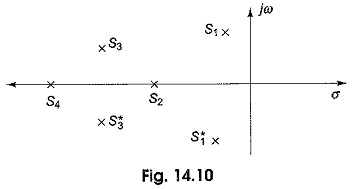
In Fig. 14.10 s1 and s3 are complex conjugate poles, whereas s2 and s4 are real poles. If the poles are real, the quadratic function is
![]()
where δ is the damping ratio and ωn is the undamped natural frequency.
The roots of the equation are
![]()
For these poles, the time domain response is given by
![]()
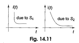
The response due to pole s4 dies faster compared to that of s2 as shown in Fig. 14.11.
s1 and s3 constitute complex conjugate poles. If the poles are complex conjugate, then the quadratic function is
![]()
The roots are
![]()
For these poles, the time domain response is given by
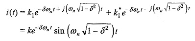
From the above equation, we can conclude that the response for the conjugate poles is damped sinusoid. Similarly, s3, s3* are also a complex conjugate pair. Here the response due to s3 dies down faster than that due to s1 as shown in Fig. 14.12.

Consider a network having transfer admittance Y(s). If the input voltage V(s) is applied to the network, the corresponding current is given by
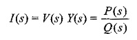
This may be taken as
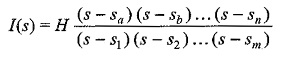
where H is the scale factor.
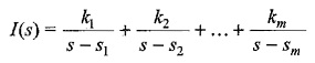
By taking the partial fractions, we get
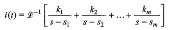
The time domain response can be obtained by taking the inverse transform
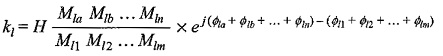
Any of the above coefficients can be obtained by using Heavisides method. To find the coefficient kl
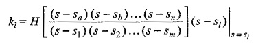
Here sl, sm, sn are all complex numbers, the difference of (sl – sn) is also a complex number.
![]()
Hence
Similarly, all coefficients k1,k2,….km may be obtained, which constitute the
magnitude and phase angle.
The residues may also be obtained by Poles and Zeros of Time Domain Response in the following way.
- Obtain the pole zero plot for the given network function.
- Measure the distances Mla, Mlb,….,Mln of a given pole from each of the other zeros.
- Measure the distances Ml1, Ml2,….,Mlm of a given pole from each of the other poles.
- Measure the angle Φla, Φlb,….,Φln of the line joining that pole to each of the other zeros.
- Measure the angle Φl1, Φl2,….,Φlm of the line joining that pole to each of the
other poles. - Substitute these values in required residue equation.
Amplitude and Phase Response from Pole Zero Plot:
The steady state response can be obtained from the pole zero plot, and it is given by
![]()
where M(ω) is the amplitude
Φ(ω) is the phase
These amplitude and phase responses are useful in the design and analysis of network functions. For different values of ω, corresponding values of M(ω) and Φ(ω) can be obtained and these are plotted to get amplitude and phase response of the given network.