Transistor Hybrid Model:

The basic assumption in arriving at a transistor linear model or equivalent circuit is that the variations about the operating or quiescent point are small and, therefore, the transistor parameters can be considered constant over the small range of operation.

Many transistor models have been proposed, each one hav­ing its particular merits and demerits. The transistor model presented here, is given in terms of the h parameters, which are real numbers at audio frequencies, are easy to measure, can also be obtained from the static characteristics of a transistor, and are particularly convenient to use in analysis and design of circuit. Furthermore, a set of h parameters is specified for many transis­tors by the manufacturers.

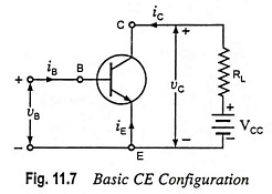
To derive a hybrid model for a transistor, let us consider the basic CE amplifier circuit given in Fig. 11.7. The variables i_B, i_C, v_B and v_C represent the total instantaneous values of currents and voltages. We may select the input current i_B and output voltage v_C as independent variables. Since input voltage v_B is some function f₁ of i_B and v_C and output current i_C is another function f₂ of i_B and v_C, we may write

Making a Taylor’s series expansion of Eqs. (11.3) and (11.4) about the zero signal operating point (I_B, V_C) and neglecting higher-order terms we have

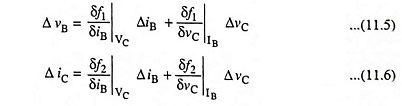
where partial derivatives δf₁/δi_B and δf₂/δi_B are taken, keeping collector voltage V_C constant while partial derivates δf₁/δv_C and δf₂/δv_C are taken, keeping base current I_B constant.

The quantities Δv_B, Δv_C, Δi_B and Δi_C represent the small-signal (incremental) base and collector voltages and currents and may be represented as v_b, v_c, i_b, and i_c respectively as per standard notations. We may now write Eqs. (11.5) and (11.6) as below

The partial derivatives of Eq. (11.9) define the h parameters for the transistor in common-emitter (CE) configuration.

Equations (11.7) and (11.8) are found to be of exactly the same form as Eqs. (11.1) and (11.2) hence, the model shown in Fig. 11.4 can be used to represent a transistor.

The common-emitter (CE), common-base (CB), and common-collector (CC) configurations, their Transistor Hybrid Model and their terminal volt-ampere equations are summarized in Table 11.2.

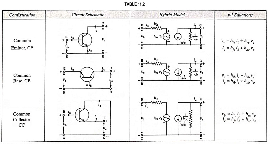
The circuits and equations in Table 11.2 are valid for either an N-P-N or P-N-P transistor and are independent of the type of load or biasing method.