Optimal Load Flow Solution:
The problem of optimal real power dispatch has been treated in the earlier section using the approximate loss formula. This section presents the more general problem of real and reactive power flow so as to minimize the instantaneous operating costs. It is a static optimization problem with a scalar objective function (also called cost function). The solution technique given here was first given by Dommel and Tinney. It is based on Optimal Load Flow Solution by the NR method, a first order gradient adjustment algorithm for minimizing the objective function and use of penalty functions to account for inequality constraints on dependent variables.
The problem of unconstrained Optimal Load Flow Solution is first tackled. Later the inequality constraints are introduced, first on control variables and then on dependent variables.
Optimal Power Flow without Inequality Constraints:
The objective function to be minimized is the operating cost

subject to the load flow equations
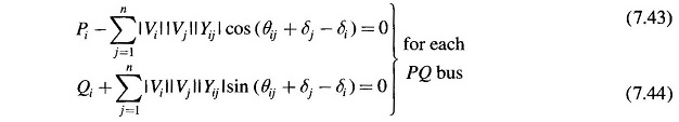
and

It is to be noted that at the ith bus
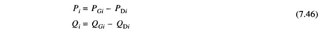
where PDi and QDi are load demands at bus i.
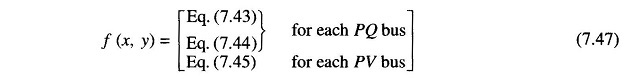
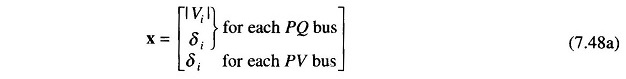
Equations (7.43), (7.44) and (7.45) can be expressed in vector form
where the vector of dependent variables is
and the vector of independent variables is
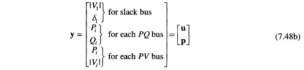
In the above formulation, the objective function must include the slack bus power.
The vector of independent variables y can be partitioned into two parts – a vector u of control variables which are to be varied to achieve optimum value of the objective function and a vector p of fixed or disturbance or uncontrollable Parameters. Control parameters may be voltage magnitudes on PV buses, PGi at buses with controllable power, etc.
The optimization problem can now be restated as

subject to equality constraints
![]()
To solve the optimization problem, define the Lagrangian function as
![]()
where λ is the vector of Lagrange multipliers of same dimension as f (x, u, p). The necessary conditions to minimize the unconstrained Lagrangian function are
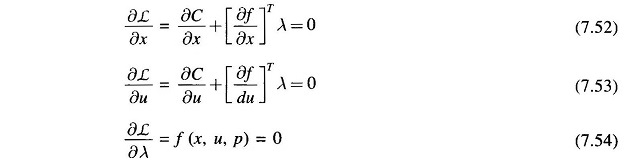
Equation (7.54) is obviously the same as the equality constraints. The expressions for δC/δx and δf/δu as needed in Eqs. (7.52) and (7.53) are rather involved. It may however be observed by comparison that δf/δx = Jacobian matrix [same as employed in the NR method of load flow solution; the expressions for the elements of Jacobian].
Equations (7.52), (7.53) and (7.54) are non-linear algebraic equations and can only be solved iteratively. A simple yet efficient iteration scheme, that can by employed, is the steepest descent method (also called gradient method).
The basic technique is to adjust the control vector u, so as to move from one feasible solution point (a set of values of x which satisfies Eq. (7.54) for given u and p; it indeed is the load flow solution) in the direction of steepest descent (negative gradient) to a new feasible solution point with a lower value of objective function. By repeating these moves in the direction of the negative gradient, the minimum will finally be reached.
The computational procedure for the gradient method with relevant details is given below:
Step 1: Make an initial guess for u, the control variables.
Step 2: Find a feasible load flow solution from Eq. (7.54) by the NR iterative method. The method successively improves the solution x as follows.
![]()
where Δx is obtained by solving the set of linear equations:
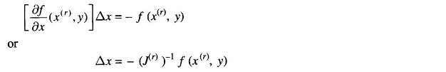
The end results of Step 2 are a feasible solution of x and the Jacobian matrix.
Step 3: Solve Eq. (7.52) for

Step 4: Insert λ from Eq. (7.55) into Eq. (7.53), and compute the gradient

It may be noted that for computing the gradient, the Jacobian J = δf/δx is already known from the Optimal Load Flow Solution (step 2 above).
Step 5: If Δζ equals zero within prescribed tolerance, the minimum has been reached. Otherwise,
Step 6: Find a new set of control variables
![]()
Where
![]()
Here Δu is a step in the negative direction of the gradient. The step size is adjusted by the positive scalar α.
Steps 1 through 5 are straightforward and pose no computational problems. Step 6 is the critical part of the algorithm, where the choice of α is very important. Too small a value of α guarantees the convergence but slows down the rate of convergence; too high a value causes oscillations around the minimum. Several methods are available for optimum choice of step size.
Inequality Constraints on Control Variables:
Though in the earlier discussion, the control variables are assumed to be unconstrained, the permissible values are, in fact, always constrained,
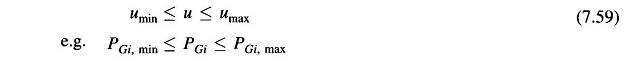
These inequality constraints on control variables can be easily handled. If the correction Δui in Eq. (7.57) causes ui to exceed one of the limits, ui is set equal to the corresponding limit, i.e.
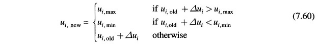
After a control variable reaches any of the limits, its component in the gradient should continue to be computed in later iterations, as the variable may come within limits at some later stage.
In accordance with the Kuhn-Tucker theorem, the necessary conditions for minimization of ζ under constraint (7.59) are:
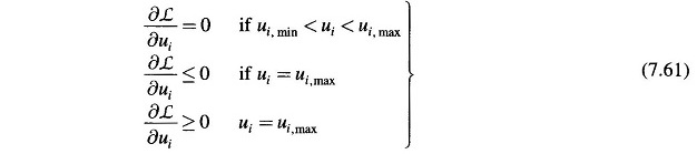
Therefore, now, in step 5 of the computational algorithm, the gradient vector has to satisfy the optimality condition (7.61).
Inequality Constraints on Dependent Variables:
Often, the upper and lower limits on dependent variables are specified as
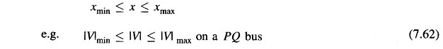
Such inequality constraints can be conveniently handled by the penalty function method. The objective function is augmented by penalties for inequality constraints violations. This forces the solution to lie sufficiently close to the constraint limits, when these limits are violated. The penalty function method is valid in this case, because these constraints are seldom rigid limits in the strict sense, but are in fact, soft limits (e.g. |V| ≤ 1.0 on a PQ bus really means V should not exceed 1.0 too much and |V| = 1.01 may still be permissible).
The penalty method calls for augmentation of the objective function so that the new objective function becomes

Where the penalty Wj is introduced for each violated inequality constraint. A suitable penalty function is defined as

where γj is a real positive number which controls degree of penalty and is called the penalty factor.
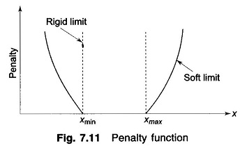
A plot of the proposed penalty function is shown in Fig. 7.11, which clearly indicates how the rigid limits are replaced by soft limits.
The necessary conditions (7.52) and (7.53) would now be modified as given below, while the conditions (7.54), i.e. load flow equations, remain unchanged.
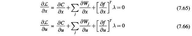
The vector δWj/δx obtained from Eq. (7.64) would contain only one non-zero term corresponding to the dependent variable xj; while δWj/δu = 0 as the penalty functions on dependent variables are independent of the control variables.
By choosing a higher value for γj, the penalty function can be made steeper so that the solution lies closer to the rigid limits; the convergence, however, will become poorer. A good scheme is to start with a low value of γj and to increase it during the optimization process, if the solution exceeds a certain tolerance limit.
This section has shown that the NR method of load flow can be extended to yield the optimal load flow solution that is feasible with respect to all relevant inequality constraints. These solutions are often required for system planning and operation.