Numerical Solution of Swing Equation:
Numerical Solution of Swing Equation – In most practical systems, after machine lumping has been done, there are still more than two machines to be considered from the point of view of system stability. Therefore, there is no choice but to solve the swing equation of each machine by a numerical technique on the digital computer. Even in the case of a single machine tied to infinite bus bar, the critical clearing time cannot be obtained from equal area criterion and we have to make this calculation Numerical Solution of Swing Equation. There are several sophisticated methods now available for the Numerical Solution of Swing Equation including the powerful Runge-Kutta method. Here we shall treat the point-by-point method of solution which is a conventional, approximate method like all numerical methods but a well tried and proven one. We shall illustrate the point-by-point method for one machine tied to infinite bus bar. The procedure is, however, general and can be applied to every machine of a multimachine system.
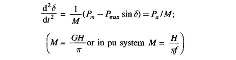
Consider the swing equation
The solution δ(t) is obtained at discrete intervals of time with interval spread of Δt uniform throughout. Accelerating power and change in speed which are continuous functions of time are discretized as below:
- The accelerating power Pa computed at the beginning of an interval is assumed to remain constant from the middle of the preceding interval to the middle of the interval being considered as shown in Fig. 12.38.
- The angular rotor velocity ω = dδ/dt (over and above synchronous velocity ωs) is assumed constant throughout any interval, at the value computed for the middle of the interval as shown in Fig. 12.38.
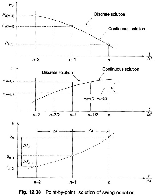
In Fig. 12.38, the numbering on t/Δt axis pertains to the end of intervals. At the end of the (n-1)th interval, the acceleration power is
![]()
where δn-1 has been previously calculated. The change in velocity (ω = dδ/dt), caused by the Pa(n-1), assumed constant over Δt from (n-3/2) to (n-1/2) is
![]()
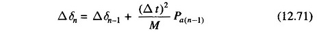
The change in δ during the (n-1)th interval is
![]()
and during the nth interval
![]()
Subtracting Eq. (12.70a) from Eq. (12.70b) and using Eq. (12.69), we get
Using this, we can write
![]()
The process of computation is now repeated to obtain Pa(n),Δδn+1 and δn+1. The time solution in discrete form is thus carried out over the desired length of time, normally 0.5 s. Continuous form of solution is obtained by drawing a smooth curve through discrete values as shown in Fig. 12.38. Greater accuracy of solution can be achieved by reducing the time duration of intervals.
The occurrence or removal of a fault or initiation of any switching event causes a discontinuity in accelerating power Pa. If such a discontinuity occurs at the beginning of an interval, then the average of the values of Pa before and after the discontinuity must be used. Thus, in computing the increment of angle occurring during the first interval after a fault is applied at t = 0, Eq. (12.71) becomes
![]()
where Pa0+ is the accelerating power immediately after occurrence of fault. Immediately before the fault the system is in steady state, so that Pa0-= 0 and δ0 is a known value. If the fault is cleared at the beginning of the nth interval, in calculation for this interval one should use for Pa(n-1) the value 1/2[Pa(n-1)- + Pa(n-1)+], where Pa(n-1)- is the accelerating power immediately before clearing and Pa(n-1)+ is that immediately after clearing the fault. If the discontinuity occurs at the middle of an interval, no special procedure is needed. The increment of angle during such an interval is calculated, as usual, from the value of Pa at the beginning of the interval.