Optimal Two Area Load Frequency Control:

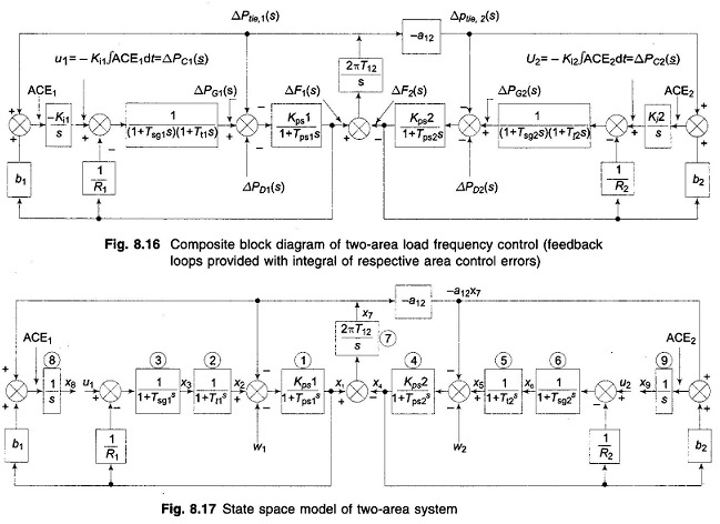
Modern control theory is applied in this section to design an Optimal Two Area Load Frequency Control for a two-area system. In accordance with modem control terminology ΔP_c1 and ΔP_C2 will be referred to as control inputs u₁ and u₂. In the conventional approach u₁ and u₂ were provided by the integral of ACEs.

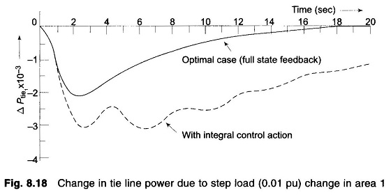
In modern control theory approach u₁ and u₂ will be created by a linear combination of all the system states (full state feedback). For formulating the state variable model for this purpose the conventional feedback loops are opened and each time constant is represented by a separate block as shown in Fig. 8.17. State variables are defined as the outputs of all blocks having either an integrator or a time constant. We immediately notice that the system has nine state variables.

Before presenting the Optimal Two Area Load Frequency Control design, we must formulate the state model. This is achieved below by writing the differential equations describing each individual block of Fig. 8.17 in terms of state variables (note that differential equations are written by replacing s by d/dt).

Comparing Figs. 8.18 and 8.19,

For Block 1

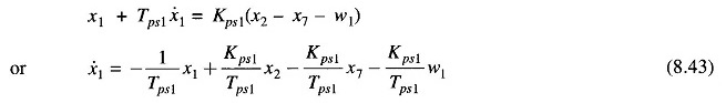
For Block 2

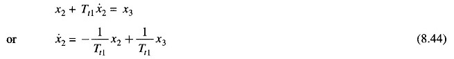
For Block 3

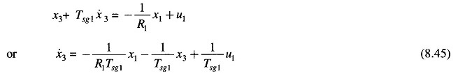
For Block 4

For Block 5

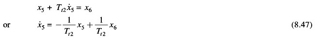
For Block 6

For Block 7

For Block 8

For Block 9

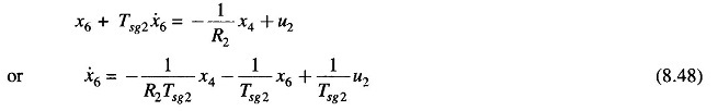
The nine equations (8.43) to (8.51) can be organized in the following vector matrix form

Where

• x = [x₁ x₂ … x₉]^T = state vector
• u = [u₁ u₂]^T = control vector
• w = [w₁ w₂]^T = disturbance vector

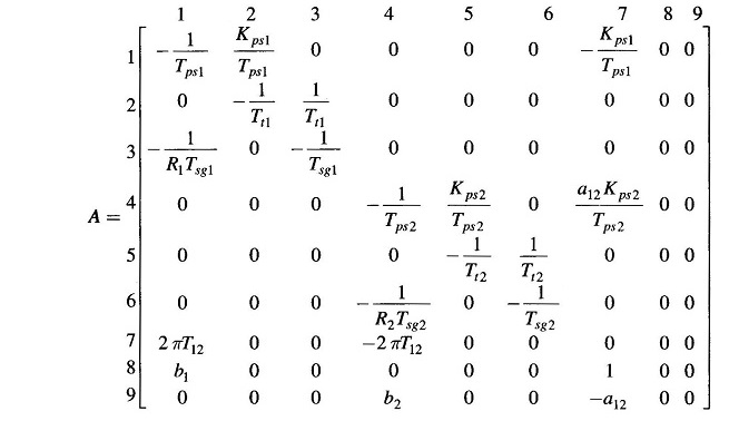
while the matrices A, B and F are defined below:

In the conventional control scheme of Fig. 8.17, the control inputs u₁ and u₂ are constructed as under from the state variables x₈ and x₉ only.

In the Optimal Two Area Load Frequency Control scheme the control inputs u₁ and u₂ are generated by means of feedbacks from all the nine states with feedback constants to be determined in accordance with an optimality criterion.

Examination of Eq. (8.52) reverals that our model is not in the standard form employed in Optimal Two Area Load Frequency Control theory. The standard form is

which does not contain the disturbance term Fw present in Eq. (8.52). Furthermore, a constant disturbance vector w would drive some of the system states and the control vector u to constant steady values; while the cost function employed in Optimal Two Area Load Frequency Control requires that the system state and control vectors have zero steady state values for the cost function to have a minimum.

For a constant disturbance vector w, the steady state is reached when

in Eq. (8.52); which then gives

Defining x and u as the sum of transient and steady state terms, we can write

Substituting x and u from Eqs. (8.54) and (8.55) in Eq. (8.52), we have

By virtue of relationship (8.53), we get

This represents system model in terms of excursion of state and control vectors from their respective steady state values.

For full state feedback, the control vector u is constructed by a linear combination of all states, i.e.

where K is the feedback matrix.

Now

For a stable system both x’ and u’ go to zero, therefore

Hence

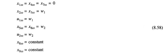
Examination of Fig. 8.17 easily reveals the steady state values of state and control variables for constant values of disturbance inputs w₁ and w₂. These are

The values of X_8ss and X_9ss depend upon the feedback constants and can be determined from the following steady state equations:

The feedback matrix K in Eq. (8.57b) is to be determined so that a certain performance index (PI) is minimized in transferring the system from an arbitrary initial state x'(0) to origin in infinite time (i.e. x'(∞) = 0). A convenient PI has the quadratic form

The matrices Q and R are defined for the problem in hand through the following design considerations:

• • Excursions of ACEs about the steady values (x′₇ + b₁x′₁; – a₁₂x′₇ + b₂x′₄) are minimized. The steady values of ACEs are of course zero.
• Excursions of ∫ACE dt about the steady values (x’₈, x’₉) are minimized. The steady values of ∫ACE dt are, of course, constants.
• Excursions of the control vector (u’₁, u’₂) about the steady value are minimized The steady value of the control vector is, of course, a constant. This minimization is intended to indirectly limit the control effort within the physical capability of components. For example, the steam valve cannot be opened more than a certain value without causing the boiler pressure to drop severely.

With the above reasoning, we can write the PI as

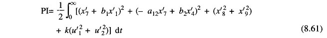
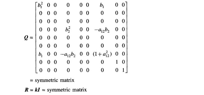
From the PI of Eq.(8.61),Q and R can be recognized as

Determination of the feedback matrix K which minimizes the above PI is the standard optimal regulator problem. K is obtained from solution of the reduced matrix Riccati equation (a set of linear algebraic equations) given below.

The acceptable solution of K is that for which the system remains stable. Substituting Eq. (8.57b) in Eq. (8.56), the system dynamics with feedback is defined by

For stability all the eigenvalues of the matrix (A – BK) should have negative real parts.

For illustration we consider two identical control areas with the following system parameters:

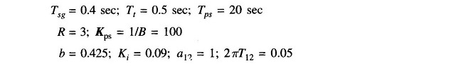
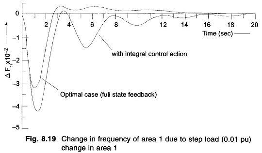
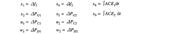
Computer solution for the feedback matrix K is presented below, while the system dynamic response is plotted in Figs. 8.18 and 8.19. These figures also give for comparison the dynamic response for the case of integral control action only. The improvement in performance achieved by the optimal controller is evident from these figures.

As the control areas extend over vast geographical regions, there are two ways of obtaining full state information in each area for control purposes.

• Transport the state information of the distant area over communication This is, of course, expensive.
• Generate all the states locally (including the distant states) by means of `observer’ or ‘Kalman filter’ by processing the local output signal. An `observer’ being itself a high order system, renders the overall system highly complex and may, in fact, result in impairing system stability and dynamic response which is meant to be improved through optimal control.

Because of the above mentioned difficulties encountered in implementation of an optimal control load frequency scheme, it is preferably to use a sub­optimal scheme employing only local states of the area. The design of such structurally constrained optimal control schemes is beyond the scope of this book. The conventional control scheme of Fig. 8.16 is, in fact, the local output feedback scheme in which feedback signal derived from changes in local frequency and tie line power is employed in each area.