Phase Margin Optimum:

The method can be based on the phase margin in which the controller is designed to provide a minimum phase margin. The design makes use of Bode plots. The ratio of time constants can be decided depending upon the phase margin required, which directly influences the damping. Therefore this method has an advantage over the previous one. As the damping factor increases the phase margin also increases. Therefore a clear dependence of these quantities and the effect of the ratio of time constants on the time response of the system is clearly brought out in the following, so that a proper design of the controller to give the desired performance can be made.

The same example as above is taken here also. The plant has a transfer function

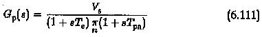
A PID controller is designed to improve the performance. The transfer func­tion of the controller is given by

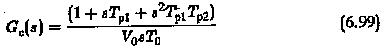
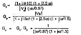
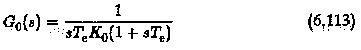
The zeros of G_c(s) are the same as the dominant poles of G_p(s), so that they compensate the large time constants of the plant. The open loop transfer function is

The design based on magnitude optimum gave a controller having its inte­grative time constant equal to twice the uncompensated time constant of the plant, i.e., T₀ = 2T_e.

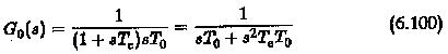
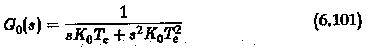
To design a controller based on phase margin the ratio of time constants is T₀/T_e is assumed to be K₀. Using this ratio we have

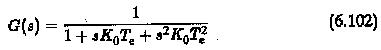
The closed loop transfer function

In the frequency domain

The phase margin of the system can be obtained as

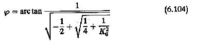
If the phase angle of the transfer function is φ_c, the the phase margin is

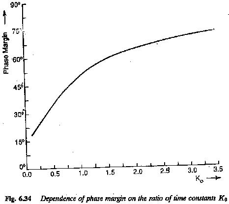
Depending on the value of required φ the value of K_o can be chosen. For a system having a known value of K₀ the phase margin is fixed. The method based on magnitude optimum assigns a value of 2 for K₀ and the corresponding phase margin is 65°.

In the present method there is a flexibility in the choice of K₀. The relation between K₀ and φ is depicted in Fig. 6.34. From this it can be concluded that the integration time constant actually decides the system improvement or its damping and this is decided from the value of K₀ (ratio of time constants). Smaller the value of K₀ smaller the value of damping. At smaller phase margins the system becomes oscillatory.

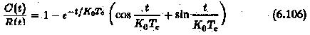
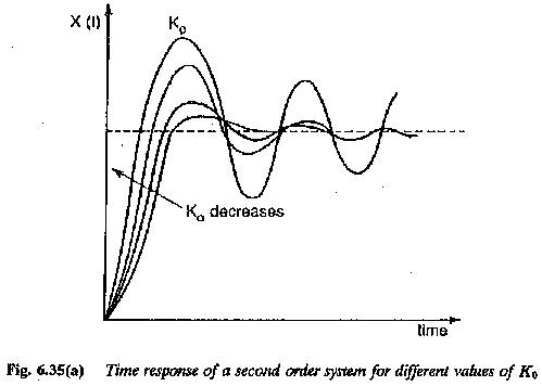
The time domain specifications can now be related to the value of K₀. These are the initial rise time, the maximum overshoot and the area under the first overshoot. The time response of the second order system for different values of K₀ is shown in Fig. 6.35. The time response can be given by equation

The damping of the response increases with the value of K₀. From the time response it can be seen that the proper value of K₀ lies between one and four. For a value of K₀ < 1.5 the t_r < 4T_e. The settling time can also be determined.

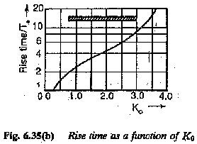
The maximum overshoot as a function of K₀ can be determined and is depicted in Fig. 6.35(b). From the figure it is clear that overshoot decreases as the value of K₀ increases. For K₀ = 1.5, % overshoot = 8.5.

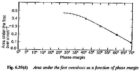
The area under the first overshoot as a function of K₀ is also shown in Fig. 6.35(c). This is obtained by evaluating the integral.

The integration results in

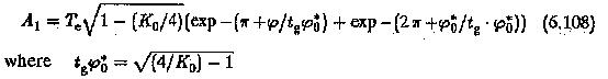
T₁/T_e drawn as a function of phase margin is depicted in Fig. 6.35(d). The first overshoot dominated for the thick portion of the characteristic,

To determine a controller of suitable frequency response a detailed dis­cussion of the effects of controller amplitude characteristic on the modified system is required. The ratio K₀ = T₀/T_e can be freely chosen while designing a controller using phase margin criterion. It has been established that the phase margin increases as the value of K₀ increases. In other words the phase of the system transfer function at the gain cross-over frequency decreases. As the phase margin is related to the damping of the system the value of K₀ and hence the value of T₀ can also be related to damping. The damping of the system is more as the value of K₀ or T₀ increases.

To have an insight into the amplitude characteristics, compensation of the plants by PI and PID controllers is examined in the following. In the former the plant transfer function has only one large time constant to be compensated and one small time constant to be uncompensated. A PI controller to modify the performance will have a time constant the same as a large time constant of the plant. The integration time of the controller T₀ however is at the designer’s choice. The transfer function of the controller is

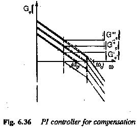
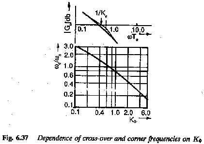
The value of T₀ can be chosen freely. Its effect on the magnitude plot of frequency response is similar to the effect gain. Thus change in value of T₀ can be regarded as change in gain and the magnitude plot moves along ordinate. For smaller values of T₀ it moves upward, increasing the value of gain cross-over frequency. The typical amplitude plots of a PI controller used to improve the performance of the plant having one large time constant, are shown in Fig. 6.36. It, clearly shows that the cross-over frequency depends upon T₀ and hence K₀. The relationship between ω_c/ω₀ and K₀ is shown in Fig. 6.37.

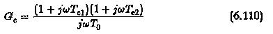
If the plant has two large time constants and one small one, the two large-time constants are compensated by a PID controller. In this case also the integration time of the controller is freely chosen. As far as the effect of T₀ on the magnitude plots is concerned it is same as in the case of PI con­troller. The magnitude plot of a PID controller having a transfer function given by

The function should have a magnitude plot such that it has a slope of 20 db/decade up to the corner frequency 1/T_e, where T_e is the uncompensated time con­stant of the plant, and later it must have a slope of 40 db/decade so that the compensations of the two time constants is effective.

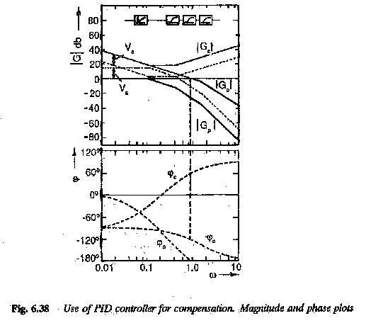
Therefore, while designing a controller its amplitude plot may be freely chosen to have the necessary gain cross-over frequency. This can be achieved by shifting the amplitude plots along the y-axis until the gain cross-over oc­curs above the required phase angle (decided by phase margin). The phase angle characteristic is the resultant of the phase angle characteristics of the plant and the controller. The proper value of T₀ is arrived at. The resul­tant open loop transfer function of the modified system can be determined. There will be a small difference between the value of K₀ determined using the asymptotic plots and the actual calculation. If the transfer function of the plant has a gain of K, the controller will have a integration time KT₀.

To summarize:

1.The transfer function of the plant to be modified is given by

where T_e ≪ T_pn,n=1,2,..

T_e is the sum of several parasitic time constants of the system.

2.The controller transfer function is chosen to compensate all T_pn. There­fore with respect to these time constants it has a form

The constant K₀ is decided so that the resultant open loop transfer function

has the specified phase margin. The closed loop transfer function has a time response of the second order system, having a damping ratio of √K₀/2.