Load Flow Analysis in Power System:
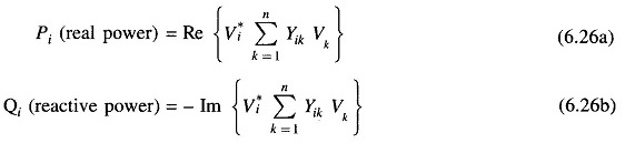
Load Flow Analysis in Power System describes, the complex power injected by the source into the ith bus of a power system is
![]()
where
- Vi is the voltage at the ith bus with respect to ground and
- Ji is the source current injected into the bus.
The Load Flow Analysis is handled more conveniently by use of Ji rather than J*i. Therefore, taking the complex conjugate of Eq. (6.24), we have
![]()
Substituting for
then we write as

Equating real and imaginary parts
In polar form

Real and reactive powers can now be expressed as
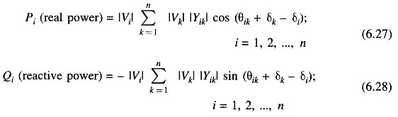
Equations (6.27) and (6.28) represent 2n power flow equations at n buses of a power system (n real power flow equations and n reactive power flow equations). Each bus is characterized by four variables; Pi, Qi, |Vi| and δi resulting in a total of 4n variables. Equations (6.27) and (6.28) can be solved for 2n variables if the remaining 2n variables are specified. Practical considerations allow a power system analyst to fix a priori two variables at each bus. The solution for the remaining 2n bus variables is rendered difficult by the fact that Eqs. (6.27) and (6.28) are non-linear algebraic equations (bus voltages are involved in product form and sine and cosine terms are present) and therefore, explicit solution is not possible. Solution can only be obtained by iterative numerical techniques.
Depending upon which two variables are specified a priori, the buses are classified into three categories.
1. PQ Bus:
At this type of bus, the net powers Pi and Qi are known (PDi and QDi are known from load forecasting and PGi and QGi are specified). The unknowns are |Vi| and δi. A pure load bus (no generating facility at the bus, i.e., PGi = QGi = 0) is a PQ bus.
2. PV Bus/Generator Bus/Voltage Controlled Bus:
At this type of bus PDi, and QDi, are known a priori and |Vi| and Pi (hence PGi) are specified. The unknowns are Qi (hence QGi) and δi.
3. Slack Bus/Swing Bus/Reference Bus:
This bus is distinguished from the other two types by the fact that real and reactive powers at this bus are not specified. Instead, voltage magnitude and phase angle (normally set equal to zero) are specified. Normally there is only one bus of this type in a given power system. The need of such a bus for a Load Flow Analysis in Power System is explained below.
In a Load Flow Analysis in Power System real and reactive powers (i.e. complex power) cannot be fixed a priori at all the buses as the net complex power flow into the network is not known in advance, the system power loss being unknown till the load flow study is complete. It is, therefore, necessary to have one bus (i.e. the slack bus) at which complex power is unspecified so that it supplies the difference in the total system load plus losses and the sum of the complex powers specified at the remaining buses. By the same reasoning the slack bus must be a generator bus. The complex power allocated to this bus is determined as part of the solution. In order that the variations in real and reactive powers of the slack bus during the iterative process be a small percentage of its generating capacity, the bus connected to the largest generating station is normally selected as the slack bus. Further, for convenience the slack bus is numbered as bus 1.
Equations (6.27) and (6.28) are referred to as static load flow equations (SLFE). By transposing all the variables on one side, these equations can be written in the vector form
![]()
where
- f = vector function of dimension 2n
- x = dependent or state vector of dimension 2n (2n unspecified variables)
- y = vector of independent variables of dimension 2n (2n independent variables which are specified a priori)
Some of the independent variables in y can be used to manipulate some of the state variables. These adjustable independent variables are called control parameters. Vector y can then be partitioned into a vector u of control parameters and a vector p of fixed parameters.
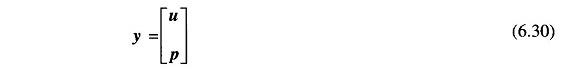
Control parameters may be voltage magnitudes at PV buses, real powers Pi, etc. The vector p includes all the remaining parameters which are uncontrollable.
For SLFE solution to have practical significance, all the state and control variables must lie within specified practical limits These limits, which are dictated by specifications of power system hardware and operating constraints, are described below:
(i) Voltage magnitude |Vi| must satisfy the inequality
![]()
The power system equipment is designed to operate at fixed voltages with allowable variations of ± (5 – 10)% of the rated values.
(ii) Certain of the δis (state variables) must satisfy the inequality constraint
![]()
This constraint limits the maximum permissible power angle of transmission line connecting buses i and k and is imposed by considerations of system stability.
(iii) Owing to physical limitations of P and/or Q generation sources, PGi and QGi are constrained as follows:
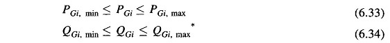
It is, of course, obvious that the total generation of real and reactive power must equal the total load demand plus losses, i.e.
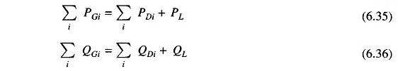
where PL and QL are system real and reactive power loss, respectively.
The Load flow problem analysis can now be fully defined as follows:
Assume a certain nominal bus load configuration. Specify PGi + jQGi at all the PQ buses (this specifies Pi + jQi at these buses); specify PGi (this specifies Pi) and |Vi| at all the PV buses. Also specify |V1| and δ1 (= 0) at the slack bus. Thus 2n variables of the vector y are specified. The 2n SLFE can now be solved (iteratively) to determine the values of the 2n variables of the vector x comprising voltages and angles at the PQ buses, reactive powers and angles at the PV buses and active and reactive powers at the slack bus. The next logical step is to compute line flows.
So far we have presented the methods of assembling a YBUS matrix and load flow equations and have defined the load flow problem in its general form with definitions of various types of buses. It has been demonstrated that load flow equations, being essentially non-linear algebraic equations, have to be solved through iterative numerical techniques.
At the cost of solution accuracy, it is possible to linearize load flow equations by making suitable assumptions and approximations so that fast and explicit solutions become possible. Such techniques have value particularly for planning studies, where load flow solutions have to be carried out repeatedly but a high degree of accuracy is not needed.
An Approximate Load Flow Solution:
Let us make the following assumptions and approximations in the load flow Eqs. (6.27) and (6.28).
- Line resistances being small are neglected (shunt conductance of overhead lines is always negligible), i.e. PL, the active power loss of the system is Thus in Eqs. (6.27) and (6.28) θik ≈ 90° and θik ≈ -90°.
- (δi – δk) is small (< π/6) so that sin (δi – δk) ≈ (δi – δk). This is justified from considerations of stability.
- All buses other than the slack bus (numbered as bus 1) are PV buses, i.e. voltage magnitudes at all the buses including the slack bus are specified.
Equations (6.27) and (6.28) then reduce to
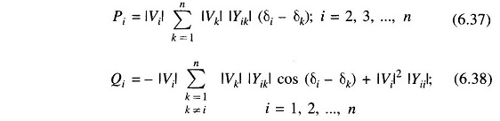
Since |Vi|s are specified, Eq. (6.37) represents a set of linear algebraic equations in δis which are (n – 1) in number as δ1 is specified at the slack bus (δ1 = 0). The nth equation corresponding to slack bus (n = 1) is redundant as the real power injected at this bus is now fully specified as

Equations (6.37) can be solved explicitly (non-iteratively) for δ2, δ3, …, δn, which, when substituted in Eq. (6.38), yields Qis the reactive power bus injections. It may be noted that the assumptions made have decoupled Eqs. (6.37) and (6.38) so that these need not be solved simultaneously but can be solved sequentially [solution of Eq. (6.38) follows immediately upon simultaneous solution of Eq. (6.37)]. Since the solution is non-iterative and the dimension is reduced to (n-1) from 2n, it is computationally highly economical.