Newton Raphson Method for Load Flow Analysis:

The Newton Raphson Method for Load Flow Analysis is a powerful method of solving non-linear algebraic equations. It works faster and is sure to converge in most cases as compared to the GS method. It is indeed the practical method of load flow solution of large power networks. Its only drawback is the large requirement of computer memory which has been overcome through a compact storage scheme. Convergence can be considerably speeded up by performing the first iteration through the GS method and using the values so obtained for starting the NR iterations. Before explaining how the NR method is applied to solve the load flow problem, it is useful to review the method in its general form.

Consider a set of n non-linear algebraic equations

Assume initial values of unknowns as x⁰₁, x⁰₂, …,x⁰_n.

Let Δx⁰₁, Δx⁰₂, …, Δx⁰_n be the corrections, which on being added to the initial guess, give the actual solution. Therefore

Expanding these equations in Taylor series around the initial guess, we have

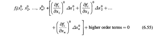
where

are the derivatives of f_i with respect to x₁, x₂, …, x_n evaluated at (x⁰₁, x⁰₂, …, x⁰_n).

Neglecting higher order terms we can write Eq. (6.55) in matrix form

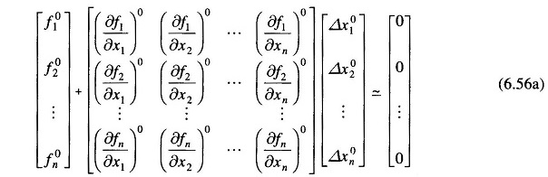
or in vector matrix form

J⁰ is known as the Jacobian matrix (obtained by differentiating the function vector f with respect to x and evaluating it at x⁰). Equation (6.56b) can be written as

Approximate values of corrections Δx⁰ can be obtained from Eq (6.57). These being a set of linear algebraic equations can be solved efficiently by triangularization and back substitution.

Updated values of x are then

or, in general, for the (r + 1)th iteration

Iterations are continued till Eq. (6.53) is satisfied to any desired accuracy, i.e.

NR Algorithm for Load flow Solution:

First, assume that all buses are PQ buses. At any PQ bus the load flow solution must satisfy the following non-linear algebraic equations

where expressions for P_i and Q_i are given in Eqs. (6.27) and (6.28). For a trial  set of variables |V_i|, δ_i, the vector of residuals f⁰ of Eq. (6.57) corresponds to

while the vector of corrections , Δx⁰ corresponds to

Equation (6.57) for obtaining the approximate corrections vector can be written for the load flow case as

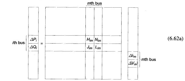
where

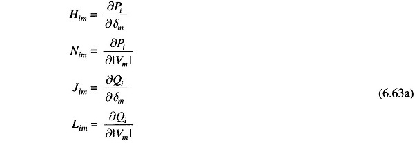
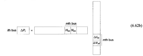
It is to be immediately observed that the Jacobian elements corresponding to the ith bus residuals and mth bus corrections are a 2 x 2 matrix enclosed in the box in Eq. (6.62a) where i and m are both PQ buses.

Since at the slack bus (bus number 1), P₁ and Q₁ are unspecified and |V₁|, δ₁ are fixed, there are no equations corresponding to Eq. (6.60) at this bus. Hence the slack bus does not enter the Jacobian in Eq. (6.62a).

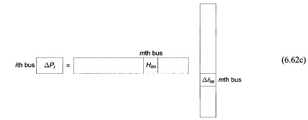
Consider Newton Raphson Method for Load Flow Analysis Formula now the presence of PV buses. If the ith bus is a PV bus, Q_i is unspecified so that there is no equation corresponding to Eq. (6.60b) for this bus. Therefore, the Jacobian elements of the ith bus become a single row pertaining to ΔP_i , i.e.

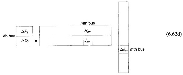
If the mth bus is also a PV bus, |V_m| becomes fixed so that Δ|V_m| = 0. We can now write

Also if the ith bus is a PQ bus while the mth bus is a PV bus, we can then write

It is convenient for numerical solution to normalize the voltage corrections

as a consequence of which, the corresponding Jacobian elements become

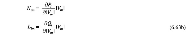
Expressions for elements of the Jacobian (in normalized form) of the load flow Eqs. (6.60a and b) are given below:

Case 1:

where

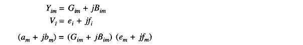
Case 2:

An important observation can be made in respect of the Jacobian by examination of the Y_BUS matrix. If buses i and m are not connected, Y_im = 0 (G_im = B_im = 0). Hence from Eqs. (6.63) and (6.64), we can write

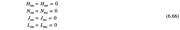
Thus the Jacobian is as sparse as the Y_BUS matrix.

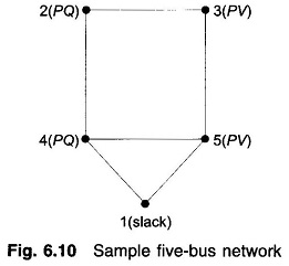
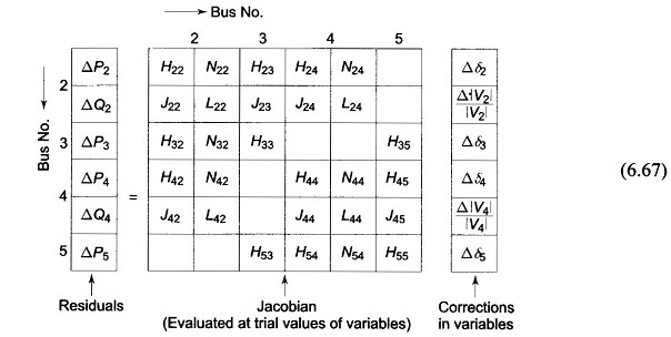
Formation of Eq. (6.62) of the NR method is best illustrated by a problem. Figure 6.10 shows a five-bus power network with bus types indicated therein. The matrix equation for determining the vector of corrections from the vector of residuals is given below.

Corresponding to a particular vector of variables [δ₂|V₂|δ₃δ₄|V₄|δ₅]^T, the vector of residuals [ΔP₂ ΔQ₂ ΔP₃ ΔP₄ ΔQ₄ ΔP₅]^T and the Jacobian (6 x 6 in this example) are computed. Equation (6.67) is then solved by triangularization and back substitution procedure to obtain the vector of corrections

Corrections are then added to update the vector of variables.

Iterative Algorithm:

Omitting programming details, the iterative algorithm for the solution of the load flow problem by the NR method is as follows:

1. With voltage and angle (usually δ = 0) at slack bus fixed, assume |V|, δ at all PQ buses and δ at all PV In the absence of any other information flat voltage start is recommended.
2. Compute ΔP_i (for PV and PQ buses) and ΔQ_i, (for all PQ buses) from (6.60a and b). If all the values are less than the prescribed tolerance, stop the iterations, calculate P₁ and Q₁ and print the entire solution including line flows.
3. If the convergence criterion is not satisfied, evaluate elements of the Jacobian using Eqs. (6.64) and (6.65).
4. Solve Eq. (6.67) for corrections of voltage angles and magnitudes.
5. Update voltage angles and magnitudes by adding the corresponding changes to the previous values and return to step 2.