RC Driving Point Impedance function:

As the name indicates, the RC networks consist of only R and C components. There is no inductor in RC networks. The RC Driving Point Impedance function is denoted as Z_RC(s). The properties of RC Driving Point Impedance function and the properties of driving point admittance function of RL network are identical. Thus the properties Z_RC(s) and Y_RL(s) are same. There are no complex poles in RC network function. The poles and zeros alternate each other and are located in left half of s plane. To understand the properties of RC network function consider a driving point impedance function of RC network as,

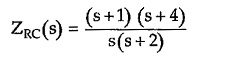
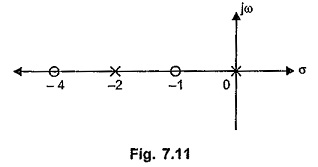
The poles are at s = 0, – 2

The zeros are at s = –1, – 4

The pole-zero plot is shown in the Fig. 7.11.

Properties of RC Driving Point Impedance Function:

Referring to the pole zero plot of Z_RC(s) function considered, the various properties of RC Driving Point Impedance function can be stated as,

1. The poles and zeros are simple. There are no multiple poles and zeros.
2. The poles and zeros are located on negative real axis.
3. The poles and zeros interlace (alternate) each other on the negative real axis.
4. We know that the poles and zeros are called critical frequencies of the The critical frequency nearest to the origin is always a pole. This may be located at the origin.
5. The critical frequency at a greatest distance away from the origin is always a zero, which may be located at ∞ also.
6. The partial fraction expansion of Z_RC(s) gives the residues which are always real and positive.
7. There is no pole located at infinity.
8. The slope of the graph of Z(σ) against σ is always negative.
9. There is no zero at the origin.
10. The value of Z_RC(s) at s=0 is always greater than the value of Z_RC(s) at s = ∞.

It can, be seen that for a Z_RC considered Z_RC(0) = ∞ while Z_RC(∞) = 1.

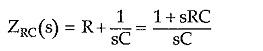
Consider a simple RC network as shown in the Fig. 7.12.

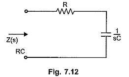
Let us plot Z_RC(σ) against σ where s = σ.

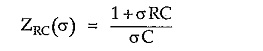
To find the slope of Z_RC(σ) against σ find d Z_RC(σ)/dσ

Thus the slope of Z_RC(σ) against σ is always negative for any value of σ.

The graph of Z(σ) against σ for the RC network function is shown in the Fig. 7.13.

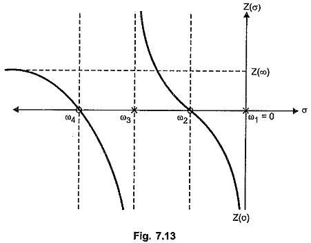
ω₁,ω₂,ω₃ and ω₄ are the critical frequencies. At the critical frequencies like ω₃, the Z(σ) changes its sign suddenly such that the slope always remains negative. The value of Z (∞) is constant so graph runs parallel to the σ axis, finally.

The nature of Z (σ) against σ graph when there is no pole at the origin is shown in the Fig. 7.14.

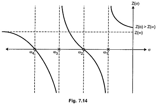
All the properties of driving point admittance function of RL network [Y_RL(s)] are exactly identical to the properties of driving point impedance function of RC network [Z_RC(s)].

Realization of Impedance Function of RC Network:

As mentioned earlier, the realization of Z_RC(s) function can be achieved using Foster I, Foster II, cauer I or cauer II form. Remember that the number of elements are not equal to highest power of s in overall Z(s) for RC networks.