Locus Diagram of RL Series Circuit:
To discuss the basis of representing a Locus Diagram of RL Series Circuit by means of a circle diagram consider the circuit shown in Fig. 8.19(a). The analytical procedure is greatly simplified by assuming that inductance elements have no resistance and that capacitors have no leakage current.
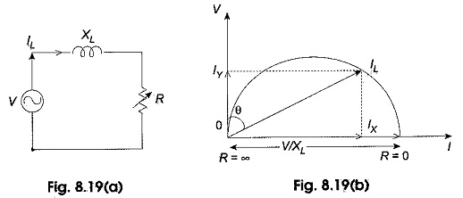
The circuit under consideration has constant reactance but variable resistance. The applied voltage will be assumed with constant rms voltage V. The power factor angle is designated by θ. If R = 0, IL is obviously equal to V/XL and has maximum value. Also I lags V by 90°. This is shown in Fig. 8.19(b). If R is increased from zero value, the magnitude of I becomes less than V/XL and θ becomes less than 90° and finally when the limit is reached, i.e. when R equals to infinity, I equals to zero and θ equals to zero. It is observed that the tip of the current vector represents a semicircle as indicated in Fig. 8.19(b).
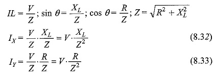
In general
![]()
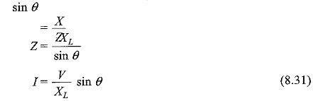
For Constant V and X, Eq. 8.31 is the polar equation of a circle with diameter V/XL. Figure 8.19(b) shows the plot of Eq. 8.31 with respect to V as reference.
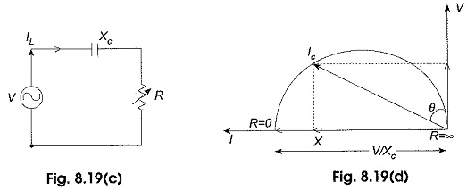
The active component of the current IL in Fig. 8.19(b) is OIL cos θ which is proportional to the power consumed in the Locus Diagram of RL Series Circuit. In a similar way we can draw the loci of current if the inductive reactance is replaced by a capacitive reactance as shown in Fig. 8.19(c). The current semicircle for the RC circuit with variable R will be on the left-hand side of the voltage vector OV with diameter V/XL as shown in Fig. 8.19(d). The current vector OIC leads V by θ°. The active component of the current ICX in Fig. 8.19(d) is OIC cos θ which is proportional to the power consumed in the RC circuit.
Circle Equations for an Locus Diagram of RL Series Circuit:
(a) Fixed reactance and variable resistance:
The X-co-ordinate and Y-co-ordinate of IL in Fig. 8.19(b) respectively are IX = IL sin θ; Iy =IL cos θ.
Where
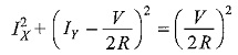
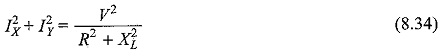
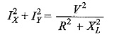
Squaring and adding Eqs. 8.32 and 8.33, we obtain
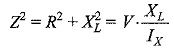
From Eq. 8.32
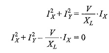
Equation 8.34 can be written as
Adding (V/2XL)2 to both sides the above equation can be written as
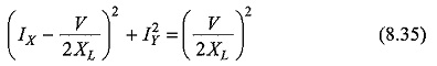
Equation 8.35 represents a circle whose radius is V/2XL and the co-ordinates of the centre are V/2XL ,0.
In a similar way we can prove that for a series RC circuit as in Fig. 8.19(c), with variable R, the locus of the tip of the current vector is a semi-circle and is given by
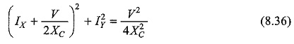
The centre has coordinates of -V/2XL ,0 and radius as V/2XL .
(b) Fixed resistance, variable reactance:
Consider the Locus Diagram of RL Series Circuit with constant resistance R but variable reactance XL as shown in Fig. 8.20(a).
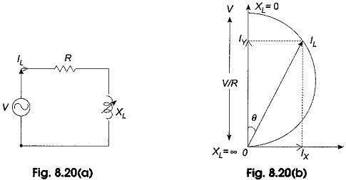
When XL = 0; IL assumes maximum value of V/R and θ = 0, the power factor of the circuit becomes unity; as the value XL is increased from zero, IL is reduced and finally where XL is α, current becomes zero and θ will be lagging behind the voltage by 90° as shown in Fig. 8,20(b). The current vector describes a semicircle with diameter V/R and lies in the right-hand side of voltage vector OV. The active component of the current OIL cos θ is proportional to the power consumed in the RL circuit.
Consider Eq. 8.34
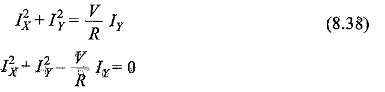
From Eq. 8.33
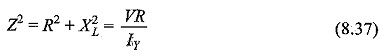
Substituting Eq 8.37 in Eq. 8.34
Adding (V/2R)2 to both sides the above equation can be written as
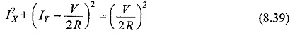
Equation 8.39 represents a circle whose radius is V/2R and the co-ordinates of the centre are 0; V/2R.
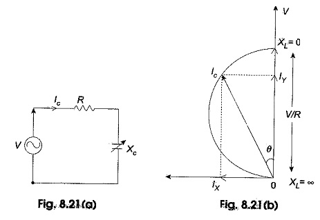
Let the inductive reactance in Fig. 8.20(a) be replaced by a capacitive reactance as shown in Fig. 8.21(a).
The current semicircle of a RC circuit with variable XC will be on the left-hand side of the voltage vector OV with diameter V/R. The current vector OIC leads V by θ°. As before, it may be proved that the equation of the circle shown in Fig. 8.21(b) is