Transmission of Waves at Transition Points:

Whenever there is an abrupt change in the parameters of a transmission line, such as an open circuit or a termination, the travelling wave undergoes a transition, part of the wave is reflected or sent back and only a portion is transmitted forward. At the Transmission of Waves at Transition Points, the voltage or current wave may attain a value which can vary from zero to two times its initial value.

The incoming wave is called the incident wave and the other waves are called the reflected and Transmission of Waves at Transition Points. Such waves are formed according to the Kirchhoff’s laws and they satisfy the line differential equations. In Fig. 8.15, is shown a typical general Transmission of Waves at Transition Points.

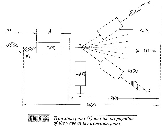
Let the transformed equations for line impedances be Z₁(s), Z₂(s) … Z_n(s), and the impedance to the ground Z_g(s) be the total impedance as seen from the transition point Z(s) and looking beyond the transition point, Z₀(s). Taking the transition point T as reference, the distance along the line away from the transition point or the line is taken as negative, so that the incoming wave towards the transition point is counted as travelling in the positive direction. Taking the lines as lossless lines, the relations can be written as follows:

In the above equation, e, i, etc. are the unprimed quantities for the incident waves, single primed quantities e’, i’, etc. are for the reflected waves and the double primed quantities e”, i”, etc. are for the transmitted waves.

At the junction point T,

From Eqs. (8.27) and (8.28), the reflected voltage wave is

and the reflected current wave is

The junction voltage e₀ and the total current i₀ are given by

The coefficients multiplying the incident quantities are called the reflection coefficients.

The impedance of any line is given by Z_k (s) + Z_k.

Hence the total impedance Z₀(s) = Z₁(s) + Z(s)

Solving the above equations, the junction potential e₀ can be written as

and the ground current, i_g = e₁/Z_g (s)

The transmitted voltage and current waves through any line K (2 < K < n) can be expressed as

The voltage drop V_K across any lumped Z_K(s) is given by

All the above functions are in the transformed form as functions of `s’ (the Laplace transform operator), and the inverse transform gives the desired time functions.

In simpler cases where the junction consists of two impedances only, the reflection and transmission coefficients become simpler and are given by reflection coefficient γ and

the transmission coefficient is (1 + γ) for voltage waves. The reflected and transmitted waves are then given by

It may be easily verified that

Solutions for lines terminated with lumped impedances can be easily worked out and the solutions for few cases are given in section 8.1.6. The above analysis of the travelling waves indicate how the waves are modified at Transmission of Waves at Transition Points. There can be doubling effect at the junction point which contributes to the over voltages in power system networks. In many overvoltage calculations, travelling wave analysis will be useful for overvoltage and overcurrent calculations.

Successive reflections and lattice diagrams:

In many problems involving short cable lengths, or lines tapped at intervals, the travelling waves encounter successive reflections at the Transmission of Waves at Transition Points. It is exceedingly difficult to calculate the multiplicity of these reflections and in his book, Bewley has given the lattice or time-space diagrams from which the motion of reflected and transmitted waves and their positions at every instant can be obtained. The principles observed in the lattice diagrams are as follows:

• all waves travel downhill, i.e. into the positive time
• the position of the wave at any instant is given by means of the time scale at the left of the lattice diagram
• the total potential at any instant of time is the superposition of all the waves which arrive at the point until the instant of time displaced in position from each other by time intervals equal to the time differences of their arrival
• attenuation is included so that the amount by which a wave is reduced is taken care of and
• the previous history of the wave, if desired can be easily. If the computation is to be carried out at a point where the operations cannot be directly placed on the lattice diagram, the anns can be numbered and the quantity can be tabulated and computed.

The above comprehensive description can be understood by considering the example shown in Fig. 8.16.

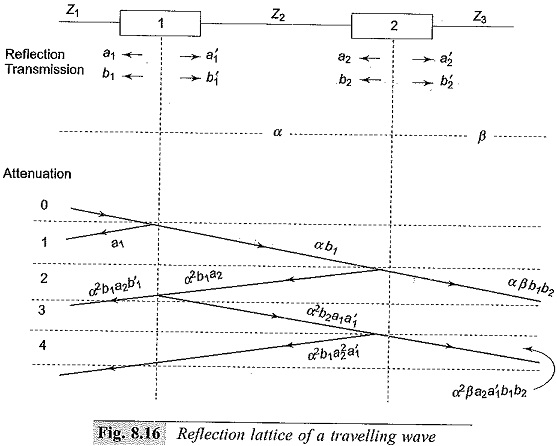
In the arrangement shown in the figure, there are two junctions 1 and 2. The travel times for the waves are different through Z₁,Z₂, and Z₃. The lines with surge impedances Z₁,Z₂, and Z₃ are connected on either side of the junctions. Let α and β be the attenuation coefficients for the two sections Z₂ and Z₃. Let a₁ and a′₁ be the reflection coefficients for the waves approaching from the left and the right at junction 1, and a₂ and a′₂ be the corresponding reflection coefficients at junction 2. Similarly, let b₁ and b′₁ be the transmission coefficients for the waves that approach from the left and the right at junction 1, and the corresponding coefficients be b₂ and b′₂ at junction 2.

To construct the lattice diagram, the position 0 is taken when the wave coming from Z₁ reaches junction 1. Junction 2 is taken to scale at the time interval equal to the travel time through the line Z₂ between the junctions 1 and 2. The diagram is drawn by choosing the suitable time  scale. The reflection and the transmission factors are marked as shown in the figure. The process of calculation is indicated on the slope of the lines in the diagram. The process can be continued for up to the required time interval.