Theory of Frequency Modulation and Phase Modulation

Theory of Frequency Modulation and Phase Modulation:

Frequency Modulation and Phase Modulation is a system in which the amplitude of the modulated carrier is kept constant, while its frequency and rate of change are varied by the modulating signal. The first practical system was put forward in 1936 as an alternative to AM in an effort to make radio transmissions more resistant to noise. Phase modulation is a similar system in which the phase of the carrier is varied instead of its frequency; as in FM, the amplitude of the carrier remains constant.

Let’s assume for the moment that the carrier of the transmitter is at its resting frequency (no modulation) of 100 MHz and we apply a modulating signal. The amplitude of the modulating signal will cause the carrier to deviate (shift) from this resting frequency by a certain amount. If we increase the amplitude (loudness) of this signal (see Figure 5-16), we will increase the deviation to a maximum of 75 kHz as specified by the FCC. If we remove the Frequency Modulation and Phase Modulation, the carrier frequency shifts back to its resting frequency (100 MHz).

We can see by this example that the deviation of the carrier is proportional to the amplitude of the modulating voltage. The shift in the carrier frequency from its resting point compared to the amplitude of the modulating voltage is called the deviation ratio (a deviation ratio of 5 is the maximum allowed in commercially broadcast FM).

The rate at which the carrier shifts from its resting point to a nonresting point is determined by the frequency of the modulating signal (the interaction between the amplitude and frequency of the modulating signal on the carrier is complex and requires the use of Bessel’s functions to analyze the results).

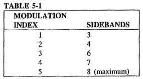
If the modulating signal (AF) is 15 kHz at a certain amplitude and the carrier shift (because of the modulating voltage) is 75 kHz, the transmitter will produce eight significant sidebands (see Table 5-1). This is known as the maximum deviation ratio:

If the frequency deviation of the carrier is known and the frequency of the modulating voltage (AF) is known, we can now establish the modulation index (MI):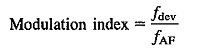

Both these terms are important because of the bandwidth limitations placed on wideband FM transmitting stations by the regulating agencies throughout the world.

Description of Systems:

The general equation of an unmodulated wave, or carrier, may be written as

where

x = instantaneous value (of voltage or current)

A = (maximum) amplitude

ω = angular velocity, radians per second (rad/s)

Φ = phase angle, rad

Note that ωt represents an angle in radians.

If any one of these three parameters is varied in accordance with another signal, normally of a lower frequency, then the second signal is called the modulation, and the first is said to be modulated by the second. Amplitude modulation, already discussed, is achieved when the amplitude A is varied. Alteration of the phase angle Φ, will yield phase modulation. If the frequency of the carrier is made to vary, frequency-modulated waves are obtained.

It is assumed that the modulating signal is sinusoidal. This signal has two important parameters which must be represented by the modulation process without distortion, specifically, its amplitude and frequency. It is understood that the phase relations of a complex modulation signal will be preserved. By the definition of frequency modulation, the amount by which the carrier frequency is varied from its unmodulated value, called the deviation, is made proportional to the instantaneous amplitude of the modulating voltage. The rate at which this frequency variation changes or takes place is equal to the modulating frequency.

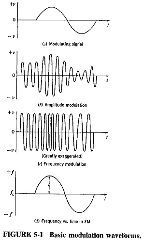
The situation is illustrated in Figure 5-1, which shows the modulating voltage and the resulting frequency-modulated wave. Figure 5-1 also shows the frequency variation with time, which can be seen to be identical to the variation with time of the modulating voltage. The result of using that modulating voltage to produce AM is also shown for comparison. As in FM, all signals having the same amplitude will deviate the carrier frequency by the same amount, for example, 45 kHz, no matter what their frequencies. All signals of the same frequency, for example, 2 kHz, will deviate the carrier at the same rate of 2000 times per second, no matter what their individual amplitudes. The amplitude of the frequency-modulated wave remains constant at all times. This is the greatest single advantage of FM.

Mathematical Representation of FM:

From Figure 5-1d, it is seen that the instantaneous frequency f of the frequency-modulated wave is given by

where

f_c = unmodulated (or average) carrier frequency

k = proportionality constant

V_m cos ω_mt = instantaneous modulating voltage (cosine being preferred for simplicity in calculations)

The maximum deviation for this particular signal will occur when the cosine term has its maximum value, ±1. Under these conditions, the instantaneous frequency will be

maximum deviation δ will be given by

The instantaneous amplitude of the FM signal will be given by a formula of the

form

where F (ω_c,ω_m) is some function of the carrier and modulating frequencies. This function represents an angle and will be called θ for convenience. The problem now is to determine the instantaneous value (i.e., formula) for this angle.

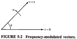
As Figure 5-2 shows, θ is the angle traced out by the vector A in time t. If A were rotating with a constant angular velocity, for example, ρ, this angle θ would be given by ρt (in radians). In this instance the angular velocity is anything but constant. It is governed by the formula for ω obtained from Equation (5-2), that is, ω = ω_c (1 + kV_m cos ω_mt). In order to find θ, ω must be integrated with respect to time. Thus

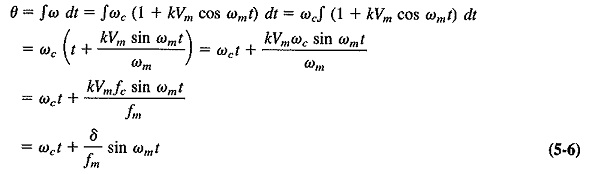
The derivation utilized, in turn, the fact that ω_c is constant, the formula ∫ cos nx dx = (sin nx)/n and Equation (5-4), which had shown that kV_mf_c = δ. Equation (5-6) may now be substituted into Equation (5-5) to give the instantaneous value of the FM voltage; therefore

The modulation index for FM, m_f, is defined as

Substituting Equation (5-8) into (5-7), we obtain

It is important to note that as the modulating frequency decreases and the modulating voltage amplitude (δ) remains constant, the modulation index increases. This will be the basis for distinguishing frequency modulation from phase modulation. Note that m_f, which is the ratio of two frequencies, is measured in radians.

Frequency Spectrum of the FM Wave:

When a comparable stage was reached with AM theory, i.e., when Equation (3-7) had been derived, it was possible to tell at a glance what frequencies were present in the modulated wave. Unfortunately, the situation is far more complex, mathematically speaking, for FM. Since Equation (5-9) is the sine of a sine, the only solution involves the use of Bessel functions. Using these, it may then be shown that Equation (5-9) may be expanded to yield

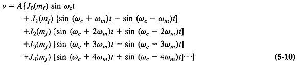
It can be shown that the output consists of a carrier and an apparently infinite number of pairs of sidebands, each preceded by J coefficients. These are Bessel functions. Here they happen to be of the first kind and of the order denoted by the subscript, with the argument m_f, J_n(m_f) may be shown to be a solution of an equation of the form

This solution, i.e., the formula for the Bessel function, is

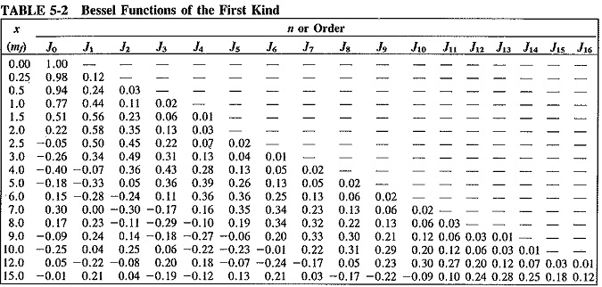
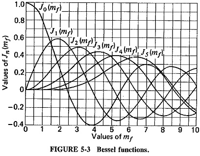
In order to evaluate the value of a given pair of sidebands or t le value of the carrier, it is necessary to know the value of the corresponding Bessel function. Separate calculation from Equation (5-12) for each case is not required since information of this type is freely available in table form, as in Table 5-2, or graphical form, as in Figure 5-3.

Observations: The mathematics of the previous discussion may be reviewed in a series of observations as follows:

Unlike AM, where there are only three frequencies (the carrier and the first two sidebands), FM has an infinite number of sidebands, as well as the carrier. They are separated from the carrier by f_m,2f_m,3f_m, . . . , and thus have a recurrence frequency of f_m.

The J coefficients eventually decrease in value as n increases, but not in any simple manner. As seen in Figure 5-3, the value fluctuates on either side of zero, gradually diminishing. Since each J coefficient represents the amplitude of a particular pair of sidebands, these also eventually decrease, but only past a certain value of The modulation index determines how many sideband components have significant amplitudes.
The sidebands at equal distances from f_c have equal amplitudes, so that the sideband distribution is symmetrical about the carrier frequency. The J coefficients occasionally have negative values, signifying a 180^° phase change for that particular pair of sidebands.

Looking down Table 5-2, as m_f increases, so does the value of a particular J coefficient, such as J₁₂.. Bearing in mind that m_f is inversely proportional to the modulating frequency, we see that the relative amplitude of distant sidebands increases when the modulation frequency is lowered. The previous statement assumes that deviation (i.e., the modulating voltage) has remained constant.
In AM, increased depth of modulation increases the sideband power and therefore the total transmitted power. In FM, the total transmitted power always remains constant, but with increased depth of modulation the required bandwidth is in To be quite specific, what increases is the bandwidth required to transmit a relatively undistorted signal. This is true because increased depth of modulation means increased deviation, and therefore an increased modulation index, so that More distant sidebands acquire significant amplitudes.
As evidenced by Equation (5-10), the theoretical bandwidth required in FM is infinite. In practice, the bandwidth used is one that has been calculated to allow for all significant amplitudes of sideband components under the most exacting This really means ensuring that, with maximum deviation by the highest modulating frequency, no significant sideband components are lopped off.
In FM, unlike in AM, the amplitude of the carrier component does not remain constant, Its J coefficient is J₀, which is a function of m_f. This may sound somewhat confusing but keeping the overall amplitude of the FM wave constant would be very difficult if the amplitude of the carrier were not reduced when the amplitude of the various sidebands increased.
It is possible for the carrier component of the FM wave to disappear completely. This happens for certain values of the modulation index, called Figure 5-3 shows that these are approximately 2.4, 5.5, 8.6, 11.8, and so on. These disappearances of the carder for specific values of m_f form a handy basis for measuring deviation.

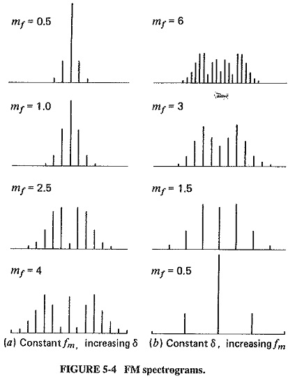
Bandwidth and required spectra: Using Table 5-2, it is possible to evaluate the size of the carrier and each sideband for each specific or value of the modulation index. When this is done, the frequency spectrum of the FM wave for that particular value of m_f may be plotted. This is done in Figure 5-4, which shows these spectrograms first for increasing deviation (f_m constant), and then for decreasing modulating frequency (δ constant). Both the table and the spectrograms illustrate the observations, especially points 2, 3, 4, and 5. It can be seen that as modulation depth increases, so does bandwidth (Figure 5-4a), and also that reduction in modulation frequency increases the number of sidebands, though not necessarily the bandwidth (Figure 5-4b). Another point shown very clearly is that although the number of sideband components is theoretically infinite, in practice a lot of the higher sidebands have insignificant relative amplitudes, and this is why they are not shown in the spectrograms. Their exclusion in a practical system will not distort the modulated wave unduly.

In order to calculate the required bandwidth accurately, the student need only look at the table to see which is the last J coefficient shown for that value of modulation index.

A rule of thumb (Carson’s rule) states that (as a good approximation) the bandwidth required to pass an FM wave is twice the sum of the deviation and the highest modulating frequency, but it must be remembered that this is only an approximation. Actually, it does give a fairly accurate result if the modulation index is in excess of about 6.

Phase Modulation:

Strictly speaking, there are two types of continuous-wave modulation; amplitude modulation and angle modulation. Angle modulation may be subdivided into two distinct types; frequency modulation and phase modulation (PM). Thus, PM and FM are closely allied, and this is the first reason for considering PM here. The second reason is somewhat more practical. It is possible to obtain frequency modulation from phase modulation by the so-called Armstrong system. Phase modulation is not used in practical analog transmission systems.

If the phase Φ, in the equation ν = A sin (ω_ct + Φ) is varied so that its magnitude is proportional to the instantaneous amplitude of the modulating voltage, the resulting wave is phase-modulated. The expression for a PM wave is

where Φ_m is the maximum value of phase change introduced by this particular modulating signal and is proportional to the maximum amplitude of this modulation. For the sake of uniformity, this is rewritten as

where m_p= Φ_m = modulation index for phase modulation.

To visualize phase modulation, consider a horizontal metronome or pendulum placed on a rotating record turntable. As well as rotating, the arm of this metronome is swinging sinusoidally back and forth about its mean point. If the maximum displacement of this swing can be made proportional to the size of the “push” applied to the metronome, and if the frequency of swing can be made equal to the number of “pushes” per second, then the motion of the arm is exactly the same as that of a phase-modulated vector. Actually, PM seems easier to visualize than FM.

Equation (5-13) was obtained directly, without recourse to the derivation required for the corresponding expression for FM, Equation (5-9). This occurs because in FM an equation for the angular velocity was postulated, from which the phase angle for ν = A sin (θ) had to be derived, whereas in PM the phase relationship is defined and may be substituted directly. Comparison of Equations (5-14) and (5-9) shows them to be identical, except for the different definitions of the modulation index. It is obvious that these two forms of angle modulation are indeed similar. They will now be compared and contrasted.

Intersystem Comparisons of Frequency Modulation and Phase Modulation:

Frequency Modulation and Phase Modulation: From the purely theoretical point of view, the difference between FM and PM is quite simple—the modulation index is defined differently in each system. However, this is not nearly as obvious as the difference between AM and FM, and it must be developed further. First the similarity will be stressed.

In phase modulation, the phase deviation is proportional to the amplitude of the modulating signal and therefore independent of its frequency. Also, since the phase modulated vector sometimes leads and sometimes lags the reference carrier vector, its instantaneous angular velocity must be continually changing between the limits imposed by Φ_m;v thus some form of frequency change must be taking place. In frequency modulation, the frequency deviation is proportional to the amplitude of the modulating voltage. Also, if we take a reference vector, rotating with a constant angular velocity which corresponds to the carrier frequency, then the FM vector will have a phase lead or lag with respect to the reference, since its frequency oscillates between f_c – δ and f_c + δ. Therefore FM must be a form of PM. With this close similarity of the two forms of angle modulation established, it now remains to explain the difference.

If we consider FM as a form of phase modulation, we must determine what causes the phase change in FM. The larger the frequency deviation, the larger the phase deviation, so that the latter depends at least to ‘a certain extent on the amplitude of the modulation, just as in PM. The difference is shown by comparing the definition of PM, which states in part that the modulation index is proportional to the modulating voltage only, with that of the FM, which states that the modulation index is also inversely proportional to the modulation frequency. This means that under identical conditions FM and PM are indistinguishable for a single modulating frequency. When the modulating frequency is changed the PM modulation index will remain constant, whereas the FM modulation index will increase as modulation frequency is reduced, and vice versa.

The practical effect of all these considerations is that if an FM transmission were received on a PM receiver, the bass frequencies would have considerably more deviation (of phase) than a PM transmitter would have given them. Since the output of a PM receiver would be proportional to phase deviation (or modulation index), the signal would appear unduly bass-boosted. Phase modulation received by an FM system would appear to be lacking in bass. This deficiency could be corrected by bass boosting the modulating signal prior to phase modulation. This is the practical difference between phase and frequency modulation.

Frequency and amplitude modulation: Frequency and amplitude modulation are compared on a different basis from that for FM and PM. These are both practical systems, quite different from each other, and so the performance and characteristics of the two systems will be compared. To begin with, frequency modulation has the following advantages:

The amplitude of the frequency-modulated wave is constant. It is thus independent of the modulation depth, whereas in AM modulation depth governs the transmitted This means that, in FM transmitters, low-level modulation may be used but all the subsequent amplifiers can be class C and therefore more efficient. Since all these amplifiers will handle constant power, they need not be capable of managing up to four times the average power, as they must in AM. Finally, all the transmitted power in FM is useful, whereas in AM most of it is in the transmitted carrier, which contains no useful information.
FM receivers can be fitted with amplitude limiters to remove the amplitude variations caused by noise, as shown in Section 5-2.2; this makes FM reception a good deal more immune to noise than AM reception.
It is possible to reduce noise still further by increasing the deviation (see Section 5-2.1). This is a feature which AM does not have, since it is not possible to exceed 100 percent modulation without causing severe distortion.
Commercial FM broadcasts began in 1940, decades after their AM counterparts. They have a number of advantages due to better planning and other considerations.

The following are the most important ones:

Standard frequency allocations (allocated worldwide by the International Radio Consultative Committee (CCIR) of the I.T.U.) provide a guard band between commercial FM stations, so that there is less adjacent-channel interference than in AM;
FM broadcasts operate in the upper VHF and UHF frequency ranges, at which there happens to be less noise than in the MF and HF ranges occupied by AM broadcasts;
At the FM broadcast frequencies, the space wave is used for propagation, so that the radius of operation is limited to slightly more than line of sight, as shown in Section 8-2.3. It is thus possible to operate several independent transmitters on the same frequency with considerably less interference than would be possible with AM.

The advantages are not all one-sided, or there would be no AM transmissions left. The following are some of the disadvantages of FM:

A much wider channel is required by FM, up to 10 times as large as that needed by This is the most significant disadvantage of FM.
FM transmitting and receiving equipment tends to be more complex, particularly for modulation and demodulation.
Since reception is limited to line of sight, the area of reception for FM is much smaller than for AM. This may be an advantage for co-channel allocations, but it is a disadvantage for FM mobile communications over a wide area. Note that this is due not so much to the intrinsic properties of FM, but rather to the frequencies employed for its transmission.