Dynamic Modelling of Induction Motor:

In general, the mechanical time-constant for any machine is much larger than the electrical time constant. Therefore, the Dynamic Modelling of Induction Motor can be simplified by neglecting the electrical transient without any loss of accuracy of results.

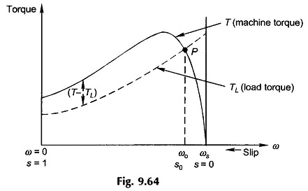
The circuit model of Induction motor holds for constant slip but would also apply for slowly varying slip as is generally the case in motor starting. Figure 9.64 shows the typical torque-slip (speed) characteristic of a Dynamic Modelling of Induction Motor and also the load torque as a function of slip (speed). Each point on (T_L-s) characteristic represents the torque (frictional) demanded by the load and motor when running at steady speed. The motor would start only if T > T_L and would reach a steady operating speed of ω₀ which corresponds to T = T_L, i.e. the intersection point P of the two torque-speed characteristics. It can be checked by the perturbation method that P is a stable operating point for the load-speed characteristic shown. If for any reason the speed becomes more than ω₀, (T – T_L) < 0 the machine-load combination decelerates and returns to the operating point. The reverse happens if the speed decreases below ω₀.

During the accelerating period

where J = combined inertia of motor and load. Now

Therefore, Eq. (9.87) modifies to

Integrating

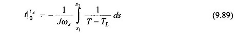
Since, the term 1/(T – T_L) is nonlinear, the integration in Eq. (9.89) must be carried out graphically (or numerically) as shown in Fig. 9.65 for the case when s₁ = 1 and s₂ = s₀.

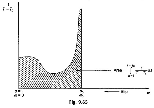
Since 1/(T – T_L) becomes ∞ at s₀, the practical integration is carried out only up to 90 or 95% of s₀ depending upon the desired accuracy.

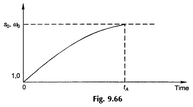
Figure 9.66 shows how slip (speed) varies with time during the acceleration period reaching the steady value of s₀(ω₀) in time t_A, the accelerating time. Because of the nonlinearity of (T – T_L) as function of slip, the slip (speed)-time curve of Fig. 9.66 is not exponential.

Starting on No-Load (T_L = 0):

In this particular case it is assumed that the machine and load friction torque T_L = 0.

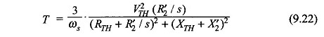
Assuming stator losses to be negligible (i.e. R₁ = 0), the motor torque as obtained from Eq. (9.22) is

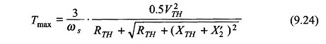
Also from Eq. (9.24)

at a slip of (Eq. (9.23))

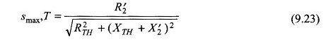
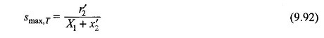
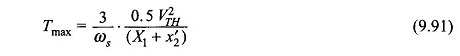
From Eqs (9.90) and (9.91),

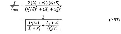
Substituting Eq. (9.92) in (9.93)

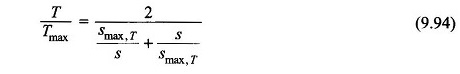
Since T_L is assumed to be zero, the motor torque itself is the accelerating torque,

i.e.

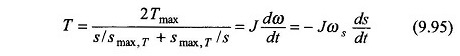
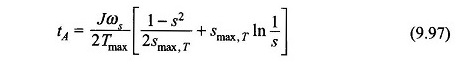
The time t_A to go from slip s₁ to s₂ is obtained upon integration of Eq. (9.95) as

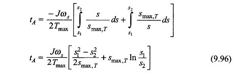
The acceleration time for the machine to reach steady speed from starting can be computed from Eq. (9.96) with s₁ = 1 and s₂ = s, i.e.

Optimum s_max,T for Minimum Acceleration Time:

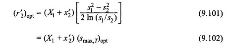
To find the optimum value of s_max,T for the Dynamic Modelling of Induction Motor to have minimum acceleration time to reach s₂ from s₁, Eq. (9.96) must be differentiated with respect to s_max,T and equated to zero. This gives

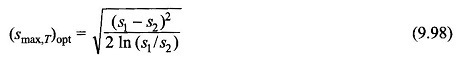
For minimum acceleration time for the machine to reach any slip s from start, the optimum value of s_max,T is given by Eq. (9.98) with s₁ = 1 and s₂ = s. Then

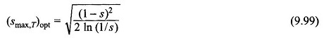
and

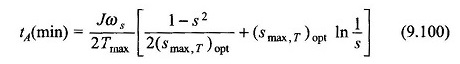
Further, to enable us to compute the optimum value of the rotor resistance to accelerate the machine to slip s₂ from s₁, Eq. (9.98) is substituted in Eq. (9.92) giving