Decoupled Load Flow Methods (DLF):
An important characteristic of any practical electric power transmission system operating in steady state is the strong interdependence between real powers and bus voltages angles and between reactive powers and voltage magnitudes. This interesting property of weak coupling between P-δ and Q-V variables gave the necessary motivation in developing the Decoupled Load Flow methods (DLF), in which P-δ and Q-V problems are solved separately.
Decoupled Newton Methods:
In any conventional Newton method, half of the elements of the Jacobean matrix represent the weak coupling referred to above, and therefore may be ignored. Any such approximation reduces the true quadratic convergence to geometric one, but there are compensating computational benefits. A large number of decoupled algorithms have been developed in the literature. However, only the most popular decoupled Newton version is presented here.
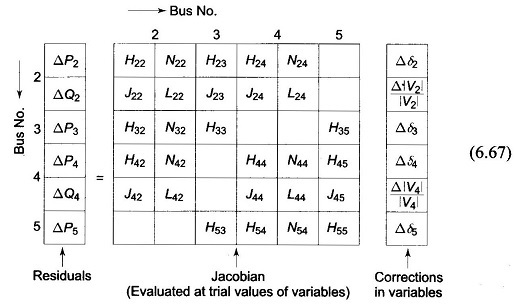
In Eq. (6.67), the elements to be neglected are submatrices [N] and [J].
The resulting decoupled linear Newton equations become
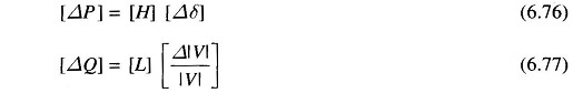
where it can be shown that
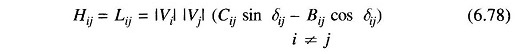
and
Equations (6.76) and (6.77) can be constructed and solved simultaneously with each other at each iteration, updating the [H] and [L] matrices in each iteration using Eqs (6.78) to (6.80). A better approach is to conduct each iteration by first solving Eq. (6.76) for Δδ, and use the updated δ in constructing and then solving Eq. (6.77) for Δ|V|. This will result in faster convergence than in the simultaneous mode.
The main advantage of the Decoupled Load Flow Methods (DLF) as compared to the NR method is its reduced memory requirements in storing the Jacobean. There is not much of an advantage from the point of view of speed since the time per iteration of the DLF is almost the same as that of NR method and it always takes more number of iterations to converge because of the approximation.
Fast Decoupled Load Flow (FDLF):
Further physically justifiable simplifications may be carried out to achieve some speed advantage without much loss in accuracy of solution using the DLF model described in the previous subsection. This effort culminated in the development of the Fast Decoupled Load Flow (FDLF) method by B. Stott in 1974. The assumptions which are valid in normal power system operation are made as follows:
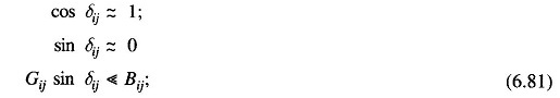
and
![]()
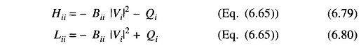
With these assumptions, the entries of the [H] and [L] submatrices will become considerably simplified and are given by
![]() and
and
![]()
Matrices [H] and [L] are square matrics with dimension (nPQ+nPV) and nPQ respectively.
Equations (6.76) and (6.77) can now be written as
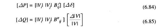
where B′ij, B″ij are elements of [- B] matrix.
Further decoupling and logical simplification of the Fast Decoupled Load Flow FDLF algorithm is achieved by:
- Omitting from [B′] the representation of those network elements that predominantly affect reactive power flows, i.e., shunt reactances and transformer off-nominal in-phase taps;
- Neglecting from [B”] the angle shifting effects of phase shifters;
- Dividing each of the Eqs. (6.84) and (6.85) by |Vi| and setting |Vj| = 1 pu in the equations;
- Ignoring series resistance in calculating the elements of [B′] which then becomes the dc approximation power flow matrix.
With the above modifications, the resultant simplified FDLF equations become
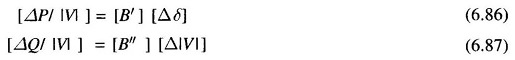
In Eqs. (6.86) and (6.87), both [B’] and [B”] are real, sparse and have the structures of [H] and [L], respectively. Since they contain only admittances, they are constant and need to be inverted only once at the beginning of the study. If phase shifters are not present, both [B’] and [B”] are always symmetrical, and their constant sparse upper triangular factors are calculated and stored only once at the beginning of the solution.
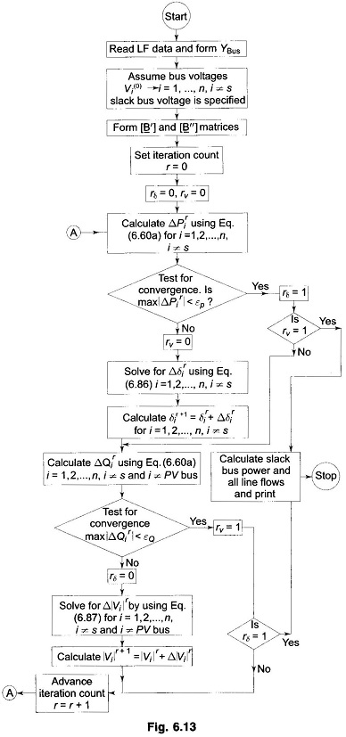
Equations (6.86) and (6.87) are solved alternatively always employing the most recent voltage values. One iteration implies one solution for [Δδ], to update [δ] and then one solution for [Δ|V|] to update [|V|] to be called 1-δ and 1-V iteration. Separate convergence tests are applied for the real and reactive power mismatches as follows:
![]()
where εP and εQ are the tolerances.
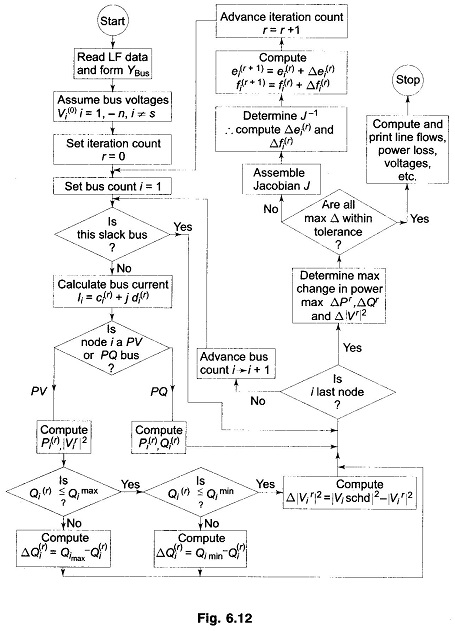
A flow chart giving FDLF algorithm is presented in Fig. 6.13.