Two Reaction Model of Salient Pole Synchronous Machine:
In a Two Reaction Model of Salient Pole Synchronous Machine, the flux established by a mmf wave is independent of the spatial position of the wave axis with respect to the field pole axis. On the other hand, in a salient-pole machine as shown in the cross-sectional view of Fig. 8.52, the permeance offered to a mmf wave is highest when it is aligned with the field pole axis (called the direct-axis or d-axis) and is lowest when it is oriented at 90° to the field pole axis (called the quadrature axis or q-axis).
Though the field winding in a Two Reaction Model of Salient Pole Synchronous Machine is of concentrated type, the B-wave produced by it is nearly sinusoidal because of the shaping of pole-shoes (the air-gap is least in the centre of the poles and progressively increases on moving away from the centre). Equivalently, the Ff wave can be imagined to be sinusoidally distributed and acting on a uniform air-gap. It can, therefore, be represented as space vector F̅f. As the rotor rotates, F̅f is always oriented along the d-axis and is presented with the d-axis permeance. However in case of armature reaction the permeance presented to it is far higher when it is oriented along the d-axis then it is oriented along the q-axis.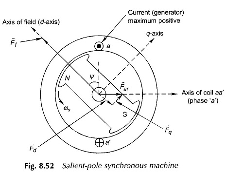
Figure 8.52 shows the relative spatial location of F̅f and F̅ar at the time instant when current (generating) in phase a is maximum positive and is lagging E̅f (excitation emf due to F̅f) by angle ψ. As angle ψ varies, the permeance offered to F̅ar , the armature reaction mmf, varies because of a change in its spatial position relative to the d-axis. Consequently F̅ar produces Φ̅̅ar (armature reaction flux/pole) whose magnitude varies with angle ψ (which has been seen earlier to be related to the load power factor). So long as the magnetic circuit is assumed linear (i.e. superposition holds), this difficulty can be overcome by dividing F̅ar into vectors F̅d along the d-axis and F̅q along the q-axis as shown by dotted lines in Fig. 8.52.
Figure 8.53 shows the phasor diagram corresponding to the vector diagram of Fig. 8.52. Here the d-axis is along F̅f and 90° behind it is the q-axis along E̅f. The components of I̅a and F̅ar along d- and q-axis are shown in the figure from which it is easily observed, that F̅d is produced by I̅d, the d-axis component of I̅a at 90° to E̅f and F̅q is produced by I̅q , the q-axis component of I̅a, in phase with E̅f.
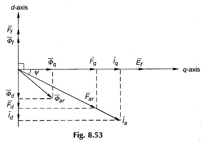
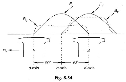
Figure 8.54 shows the relative locations of Fd, Fq and field poles and the B-waves produced by these. It is easily seen that the B-waves contain strong third-harmonic space waves. For reasons already discussed, one can proceed with the analysis on the basis of space fundamentals of Bd and Bq while neglecting harmonics.
The flux components/pole produced by the d- and q-axis components of armature reaction mmf are
![]()
![]()
The flux phasors Φ̅d and Φ̅q are also drawn in Fig. 8.53. The resultant armature reaction flux phasor Φ̅ar is now no longer in phase with F̅ar or I̅a because Pd > Pq in Eqs (8.63) and (8.64). In fact (Φ̅ar lags or leads I̅a depending upon the relative magnitudes of the d-axis, q-axis permeances.
The emfs induced by Φd and Φq are given by
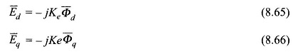
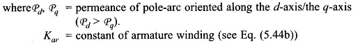
where
- Ke = emf constant of armature winding
The resultant emf induced in the machine is then
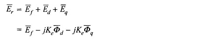
Substituting for Φ̅d and Φ̅q from Eqs (8.63) and (8.64),
![]()
Let
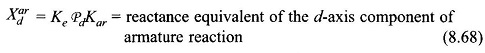
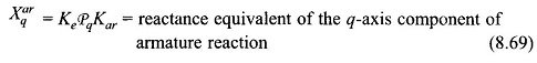
Obviously
![]()
It then follows from Eq. (8.67) that
![]()
Also for a realistic machine
![]()
Combining Eqs (8.71) and (8.72)
![]()
Define
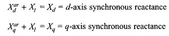
It is easily seen that
![]()
Equation (8.73) can now be written as
![]()
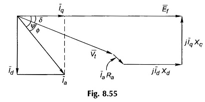
The phasor diagram depicting currents and voltages as per Eq. (8.75) is drawn in Fig. 8.55 in which δ is the angle between the excitation emf Ef and the terminal voltage Vt.
Analysis of Phasor Diagram of Salient Pole Synchronous Generator:
In the phasor diagram of Two Reaction Model of Salient Pole Synchronous Machine Fig. 8.55, the angle ψ=Φ+δ is not known for a given Vt, Ia and Φ. The location of Ef being unknown, Id and lq cannot be found which are needed to draw the phasor diagram. This difficulty is overcome by establishing certain geometric relationships for the phasor diagrams which are drawn in Fig. 8.56(a) for the generating machine and in Fig. 8.56(b) for the motoring machine.
In Fig. 8.56(a) AC is drawn at 90° to the current phasor I̅a and CB is drawn at 90° to E̅f . Now
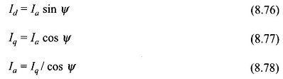
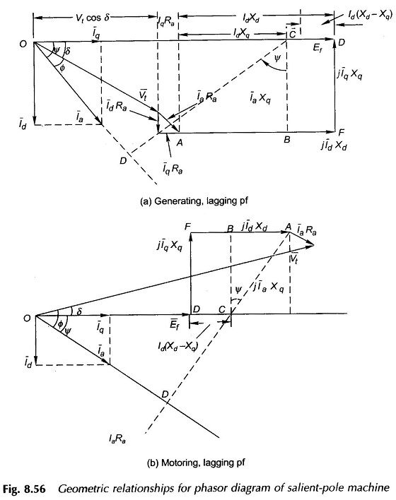
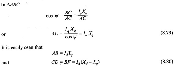
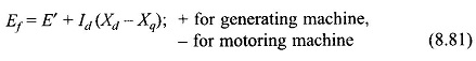
The phasor E̅f can then be obtained by extending OC by +CD for generating machine and -CD for motoring machine, where CD is given by Eq. (8.80). Let us indicate phasor OC by E̅′.
Then in terms of magnitude