Power Budget in Optical Fiber:

The term Power Budget in Optical Fiber is the relationship between the power losses in fiber links and associated equipment and the available input power to the system. The available Power Budget in Optical Fiber for a set of equipment is usually given by the. manufacturer. In some cases, the transmitted power and receiver sensitivity are specified instead. In this case the power budget is determined by subtracting the receiver sensitivity from the transmit power.

Remember that both transmit power and receive sensitivity are usually less than 1 mW; thus both numbers are likely to be negative. For example, assume:

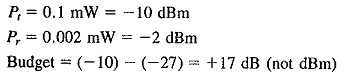
Power Budget in Optical Fiber calculations can be performed in two ways worst-case or statistically. With the worst-case approach, the values for launch power, receiver sensitivity, connector and fiber loss, and so forth, are the ones the manufacturer will never exceed. The statistical alternative uses mean or typical values to predict what will normally be seen in service. Standard deviation data is then used to predict the worst-case performance. The worst-case approach is described here.

Another term in the Power Budget in Optical Fiber is the margin for degradation of the optical components throughout their service life. The LED is the main factor, since there are common mechanisms which cause its light output to decrease over time. Because the light output falls gradually, the point at which it is “too low” is rather arbitrary. Typical values run from 1 to 3 dB. Consult the manufacturer of the equipment for the appropriate value to use. The aging margin may be built into the manufacturer’s specification for launch power.

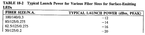
Launch power is determined by measuring the power coupled into a short piece of fiber. It is important to determine the size of fiber that was used to rate the transmit power of a particular piece of equipment. In many cases the optical fiber receptacle on a piece of equipment houses the light source. When the cable is connected to the LED, more power will be launched into large core fibers than into small ones. Table 18-2 indicates how this varies for common short-wavelength LEDs like the ones used in AMP data links. This does not apply to equipment which uses an internal fiber pigtail.

Passive Components:

Passive components are not perfect. Therefore, some of the optical energy traveling from transmitter to receiver is lost. A decrease in power levels also occurs in splitting devices, such as star couplers, as the energy arriving on one fiber is divided among several output fibers. Loss occurring in connectors and switches is proportional and is expressed in decibels. Typical values for connectors run from a few tenths of a decibel for a high-precision connector to several decibels for lower-cost varieties. Switch loss also ranges from less than 1 decibel to several decibels.

The theoretical splitting loss and the excess loss of a star coupler are usually combined to yield a maximum insertion loss. This is accommodated in the Power Budget in Optical Fiber in the same way as a connector or switch. Specified values for switches, couplers, or WDMs may or may not include the associated connectors. They should be added to the overall connector count if the loss is not included with the device.

Loss in a fiber optic cable is distributed over its length; therefore, the attenuation is expressed in decibels per kilometer (dB/km). The loss for a specific length of cable is found by multiplying its attenuation in decibels per kilometer by its length (also expressed in kilometers).

Receivers:

The detectors in optical receivers are typically larger than the common telecommunication fibers. Therefore, their sensitivity, unlike that of transmitters, does not usually vary with fiber size. As with transmitters, the loss at the connector attached to the receiver is usually included in the sensitivity rating. Receiver sensitivity is degraded by pulse spreading due to dispersion. This may be included in the specified sensitivity or described separately as a dispersion penalty. Consult the equipment manufacturer for guidance.

The basic equation for the available power (known as gain) is:

where

P_t =  transmitter launch power, dBm (average or peak)

P_r = receiver sensitivity, dBm (average or peak but same as transmitter)

P_d = dispersion penalty, dB

M_a = margin for LED aging (typically 1-3 dB)

M_s = margin for safety (typically 1-3 dB)

The loss must be less than, or equal to, the gain.

where:

l_c = length of cable, km

L_c = maximum attenuation of cable, dB/km at the wavelength of interest

N_con = number of connectors

L_con = maximum connector loss, dB

N_s = number of installation splices

N_r = number of repair splices

L_s = maximum splice loss, dB

L_pc = passive component loss, dB (couplers, switches, WDMs etc.)

The unused margin, which should not be less than zero.

Installations with losses that exceed the power budget by a small amount will still work. However, they do so by eating into the margin allocated for repair, safety, and aging. Power Budget in Optical Fiber analysis is typically not performed for each and every link in an installation. Rather, the most demanding links (longest cable, most connectors) are analyzed.

Successful installations require proper planning. With any installation, proper planning includes site surveys, detailed floor plans, bills of material, and attention to details. One detail that should not be overlooked is the power budget analysis It can pinpoint trouble spots, indicating the need for premium cable, added repeaters, or low-loss splices instead of connectors. It can also identify opportunities for cost savings through the use of higher-attenuation cable and can show when enough power is available to add reconfiguration panels for flexibility, maintenance, and growth.