Load Frequency Control of Single Area System:

Let us consider the problem of controlling the power output of the generators of a closely knit electric area so as to maintain the scheduled frequency. All the generators in such an area constitute a coherent group so that all the generators speed up and slow down together maintaining their relative power angles. Such an area is defined as a control area. The boundaries of a control area will generally coincide with that of an individual Electricity Board Company. To understand the Load Frequency Control of Single Area System, let us consider a single turbo-generator system supplying an isolated load.

Turbine Speed Governing System:

Figure 8.2 shows schematically the governing system of a steam turbine. The system consists of the following components:

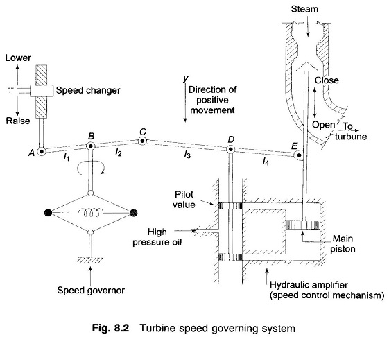
(i) Fly ball speed governor: This is the heart of the system which senses the change in speed (frequency). As the speed increases the fly balls move outwards and the point B on linkage mechanism moves downwards. The reverse happens when the speed decreases.

(ii) Hydraulic amplifier: It comprises a pilot valve and main piston Low power level pilot valve movement is converted into high power level piston valve movement. This is necessary in order to open or close the steam valve against high pressure steam.

(iii) Linkage mechanism: ABC is a rigid link pivoted at B and CDE is another rigid link pivoted at This link mechanism provides a movement to the control valve in proportion to change in speed. It also provides a feedback from the steam valve movement (link 4).

(iV) Speed changer: It provides a steady state power output setting for the turbine. Its downward movement opens the upper pilot valve so that more steam is admitted to the turbine under steady conditions (hence more steady power output). The reverse happens for upward movement of speed changer.

Model of Speed Governing System:

Assume that the system is initially operating under steady conditions—the linkage mechanism stationary and pilot valve closed, steam valve opened by a definite magnitude, turbine running at constant speed with turbine power output balancing the generator load. Let the operating conditions be characterized by

• f° = system frequency (speed)
• P°_G = generator output = turbine output (neglecting generator loss)
• y°_E = steam valve setting

We shall obtain a linear incremental model around these operating conditions.

Let the point A on the linkage mechanism be moved downwards by a small amount Δ_yA. It is a command which causes the turbine power output to change and can therefore be written as

where ΔP_C is the commanded increase in power.

The command signal ΔP_C (i.e. Δ_yE) sets into motion a sequence of events—the pilot valve moves upwards, high pressure oil flows on to the top of the main piston moving it downwards; the steam valve opening consequently increases, the turbine generator speed increases, i.e. the frequency goes up. Let us model these events mathematically.

Two factors contribute to the movement of C:

(i) Δy_A contributes — (l₂/l₁) Δy_A or -k₁Δy_A(i.e. upwards) of – k₁K_CΔP_C

(ii) Increase in frequency Δf causes the fly balls to move outwards so that B moves downwards by a proportional amount k′₂  Δf. The consequent movement of C with A remaining fixed at Δy_A is + (l₁ + l₂ / l₁) k′₂Δf = + k₂Δf

(i.e. downwards)

The net movement of C is therefore

The movement of D, Δy_D, is the amount by which the pilot value opens. It is contributed by Δy_C and Δy_E and can be written as

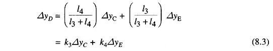
The movement Δy_D depending upon its sign opens one of the ports of the pilot valve admitting high pressure oil into the cylinder thereby moving the main piston and opening the steam valve by Δy_E. Certain justifiable simplifying assumptions, which can be made at this stage, are:

1. Inertial reaction forces of main piston and steam valve are negligible compared to the forces exerted on the piston by high pressure oil.
2. Because of (i) above, the rate of oil admitted to the cylinder is proportional to port opening Δy_D.

The volume of oil admitted to the cylinder is thus proportional to the time integral of Δy_D. The movement Δy_E is obtained by dividing the oil volume by the area of the cross-section of the piston. Thus

It can be verified from the schematic diagram that a positive movement Δy_D causes negative (upward) movement Δy_E accounting for the negative sign used in Eq. (8.4).

Taking the Laplace transform of Eqs. (8.2), (8.3) and (8.4), we get

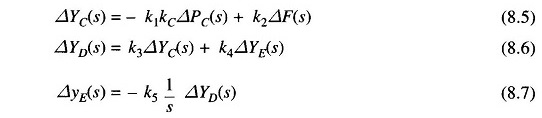
Eliminating ΔY_C(s) and ΔY_D(s), we can write

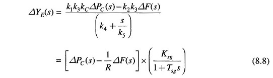
Where

• R = k₁k_C/k₂ = speed regulation of the governor
• K_sg = k₁k₃k_C/k₄ = gain of speed governor
• T_sg = 1/ k₄k₅ = time constant of speed governor

Equation (8.8) is represented in the form of a block diagram in Fig. 8.3.

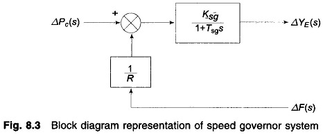
The speed governing system of a hydro-turbine is more involved. An additional feedback loop provides temporary droop compensation to prevent instability. This is necessitated by the large inertia of the penstock gate which regulates the rate of water input to the turbine. Modelling of a hydro-turbine regulating system is beyond the scope of this book.

Turbine Model:

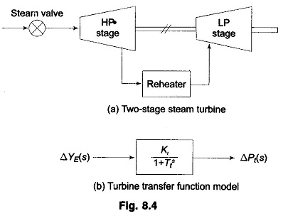
Let us now relate the dynamic response of a steam turbine in terms of changes in power output to changes in steam valve opening Δy_E. Figure 8.4a shows a two stage steam turbine with a reheat unit. The dynamic response is largely influenced by two factors, (i) entrained steam between the inlet steam valve and first stage of the turbine, (ii) the storage action in the reheater which causes the output of the low pressure stage to lag behind that of the high pressure stage. Thus, the turbine transfer function is characterized by two time constants. For ease of analysis it will be assumed here that the turbine can be modelled to have a single equivalent time constant. Figure 8.4b shows the transfer function model of a steam turbine. Typically the time constant T_t lies in the range 0.2 to 2.5 sec.

Generator Load Model:

The increment in power input to the generator-load system is

where ΔP_G = ΔP_t incremental turbine power output (assuming generator incremental loss to be negligible) and ΔP_D is the load increment.

This increment in power input to the system is accounted for in two ways:

(i) Rate of increase of stored kinetic energy in the generator rotor. At scheduled frequency (f°), the stored energy is

where P_r is the kW rating of the turbo-generator and H is defined as its inertia constant.

The kinetic energy being proportional to square of speed (frequency), the
kinetic energy at a frequency of (f° + Δf) is given by

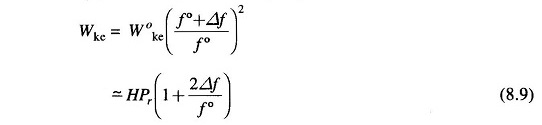
Rate of change of kinetic energy is therefore

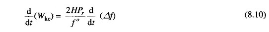
(ii) As the frequency changes, the motor load changes being sensitive to speed, the rate of change of load with respect to frequency, i.e. δP_D/δf can be regarded as nearly constant for small changes in frequency Δf and can be expressed as

where the constant B can be determined empirically. B is positive for a predominantly motor load.

Writing the power balance equation, we have

Dividing throughout by P_r and rearranging, we get

Taking the Laplace transform, we can write ΔF(s) as

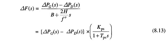
Where

• T_ps = 2H/Bf° = power system time constant
• K_ps = 1/B = power system gain

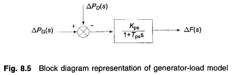
Equation (8.13) can be represented in block diagram form as in Fig. 8.5.

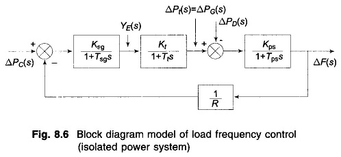
Complete Block Diagram Representation of Load Frequency Control of Single Area System of an Isolated Power System:

A complete block diagram representation of an isolated power system comprising turbine, generator, governor and load is easily obtained by combining the block diagrams of individual components, i.e. by combining Figs. 8.3, 8.4 and 8.5. The complete block diagram with feedback loop is shown in Fig. 8.6.

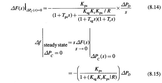
Steady States Analysis:

The model of Fig. 8.6 shows that there are two important incremental inputs to the Load Frequency Control of Single Area System -ΔP_C, the change in speed changer setting; and ΔP_D, the change in load demand. Let us consider a simple situation in which the speed changer has a fixed setting (i.e. ΔP_C = 0) and the load demand changes. This is known as free governor operation. For such an operation the steady change in system frequency for a sudden change in load demand by an amount ΔP_D (i.e. ΔP_D(s) = ΔP_D/s) is obtained as follows:

While the gain K_t is fixed for the turbine and K_ps is fixed for the power system, K_sg, the speed governor gain is easily adjustable by changing lengths of various links. Let it be assumed for simplicity that K_sg is so adjusted that

It is also recognized that K_ps = 1/B, where B = δP_D/δf / P_r (in pu MW/unit change in frequency). Now

The above equation gives the steady state changes in frequency caused by changes in load demand. Speed regulation R is naturally so adjusted that changes in frequency are small (of the order of 5% from no load to full load). Therefore, the linear incremental relation (8.16) can be applied from no load to full load. With this understanding, Fig. 8.7 shows the linear relationship between frequency and load for free governor operation with speed changer set to give a scheduled frequency of 100% at full load. The ‘droop’ or slope of this relationship is -(1/ B+(I/R)).

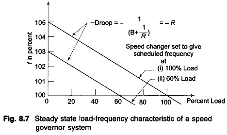
Power system parameter B is generally much smaller than 1/R (a typical value is B = 0.01 pu MW/Hz and 1/R = 1/3) so that B can be neglected in comparison. Equation (8.16) then simplifies to

The droop of the Load Frequency Control of Single Area System curve is thus mainly determined by R, the speed governor regulation.

It is also observed from the above that increase in load demand (ΔP_D) is met under steady conditions partly by increased generation (ΔP_G) due to opening of the steam valve and partly by decreased load demand due to drop in system frequency. From the block diagram of Fig. 8.6 (with K_sgK_t ≈ 1)

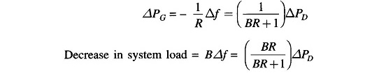
Of course, the contribution of decrease in system load is much less than the increase in generation. For typical values of B and R quoted earlier

Consider now the steady effect of changing speed changer setting (ΔP_C(s) = ΔP_C/s) with load demand remaining fixed (i.e. ΔP_D = 0). The steady state change in frequency is obtained as follows.

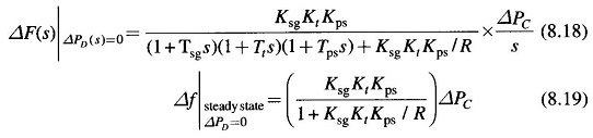
If

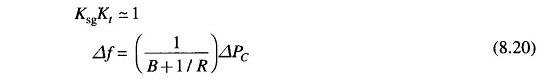
If the speed changer setting is changed by ΔP_C while the load demand changes by ΔP_D, the steady frequency change is obtained by superposition, i.e.

According to Eq. (8.21) the frequency change caused by load demand can be compensated by changing the setting of the speed changer, i.e.

Figure 8.7 depicts two load frequency plots—one to give scheduled frequency at 100% rated load and the other to give the same frequency at 60% rated load.