Classification of Active Filters:
An electric filter is often a frequency selective circuit that passes a specified band of frequencies and blocks or attenuates signals of frequencies outside this band. Classification of Active Filters are as follows.
- Analog or digital filters
- Passive or active filters
- Audio (AF) or radio (RF) filters
Analog filters are designed to process analog signals using analog techniques, while digital filters process analog signals using digital techniques. Depending on the type of elements used in their construction, filters may be classified as active or passive.
The elements used in passive filters are R, C and L. Active filters, on the other hand, employ transistors or opamps in addition to resistors and capacitors. The type of element used dictates the operating frequency range of the filter.
For example, RC filters are commonly used for audio or low frequency operation, whereas LC filters or crystal filters are employed at RF or high frequency. Because of their high Q value (figure of merit), the crystals provide stable operation at high frequency. Inductors are not used in the audio range because they are large, costly and may dissipate a lot of power. An Classification of Active Filters offers the following advantages over a passive filter.
1. Gain and frequency adjustment flexibility
Since the opamp is capable of providing a gain, the input signal is not attenuated, as in a passive filter. Also, an active filter is easier to tune.
2. No loading problem
Because of the high input resistance and low output resistance of the opamp, the active filter does not cause loading of the source or load.
3. Cost
Active filters are typically more economical than passive filters. This is because of the variety of cheaper opamps available, and the absence of inductors.
Although active filters are most extensively used in the field of communications and signal processing, they are employed in one form or another in almost all sophisticated electronic systems, radio, TV, telephones, radar, space satellites and biomedical equipment.
The most commonly used Classification of Active Filters are as follows.
- Low pass filter
- High pass filter
- Band pass filter
- Band stop filter
- All pass filter
Each of these filters uses an opamp as the active element and R, C as the passive element.
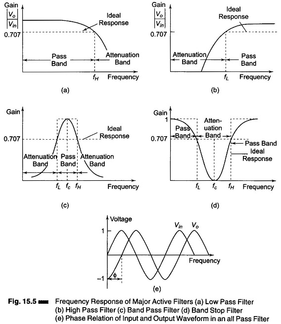
Figure 15.5 shows the frequency response characteristics of the Classification of Active Filters. The ideal response is shown by the dashed lines, while solid lines indicate the practical filter response.
A low pass filter has a constant gain from 0 Hz to a high cutoff frequency fH. Therefore, the band width is also fH.
At fH, the gain is down by 3 dbs, for f > fH, it decreases with increase in input frequency. Frequencies between 0 Hz and fH are known as pass band frequencies, while the range of frequencies beyond fH, that are attenuated, are called the stop band frequencies.
Figure 15.5(a) shows the frequency response of a low pass filter. As indicated by the dashed line, an ideal filter has a zero attenuation in its pass band and infinite attenuation in the attenuation band. However, ideal filter response is not practical because linear network cannot produce discontinuities. But, it is possible to obtain a practical response that approximates the ideal response by using special design techniques as well as precision components and high speed opamps.
Butterworth, Chebyschev, Bessel and Elliptic filters are the most commonly used practical filters for approximating the ideal response. In many low pass filter applications, it is necessary for the closed loop gain to be as close to unity as possible within the pass band.
The Butterworth filter is best suited for this application. The key characteristic of the Butterworth filter is that it has a flat pass band as well as a flat stop band. For this. reason it is sometimes called a flat-flat filter.
The Chebyschev filter has a ripple pass band and a flat stop band, while the Elliptic filter has a ripple pass band and a ripple stop band. Generally, the Elliptic filter gives the best stop band response among the three.
Figure 15.5 (b) shows a high pass filter with a stop band 0 < f < fH and a pass band f > fL, where fL is the low cutoff frequency and f is the operating frequency.
A band pass filter has a pass band between the two cutoff frequencies fH and fL, where fH > fL, and two stop bands at 0 < f < fL and f > fH. The bandwidth of the band pass filter therefore equals (fH – fL). The frequency response of the band pass filter is as shown in Fig. 15.5(c).
The band reject filter is exactly opposite to the band pass. It has a band stop between two cutoff frequencies fH and fL, and two pass bands, 0 < f < fL and f > fH. The band reject is also called a band stop or band elimination filter. The frequency response of a band stop filter is shown in Fig. 15.5(d). In this, fc is called the centre frequency, since it is approximately at the centre of the pass or stop band.
Figure 15.5(e) shows the phase shift between the input and output voltages of an all pass filter. This filter passes all frequencies equally well, i.e. the output and input voltages are equal in amplitude for all frequencies, with the phase shift between the two, a function of frequency. The highest frequency up to which the input and output amplitudes remain equal is dependent on the unity gain bandwidth of the opamp. At this frequency, however, the phase shift between the input and output is maximum. For applications where the phase shift is important, the Bessel filter which has a minimal phase shift is used, even though its cutoff characteristics are not very sharp.
As shown in Figs 15.5 (a) to (d), the actual response curve of the filters in the stop band either steadily increase or decrease with increase in frequency. The rate at which the gain of the filter changes in the stop band is determined by the order of the filter. For example, in the case of Butterworth filters, for the first order low pass filter, the gain rolls off at rate of – 20 db/decade in the stop band (f > fH). On the other hand, for the second order low pass filter the roll off rate is – 40 dB/decade and so on.
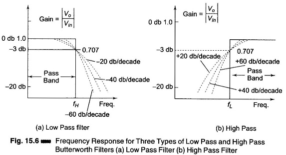
Figure 15.6 (a) shows the ideal response (solid line) and the practical (dashed lines) frequency response for three types of Butterworth low pass filters. As the roll of becomes steeper, they approach the ideal filter characteristics more closely.
By contrast, for the first order high pass filter, the gain increases at the rate of 20 db/decade in the stop band, that is, until f = fL. The increase is 40 db/ decade for the second order high pass filter and so on. Figure 15.6 (b) shows the frequency response for three types of high pass Butterworth filters.