Complex Locus of RLC Networks:
Complex Locus of RLC Networks – The network function G(s) or H(s) can be impedance function or an admittance function hence referred as immitance function. In the frequency domain G(jω) or H(jω) can be represented in rectangular form or polar form.
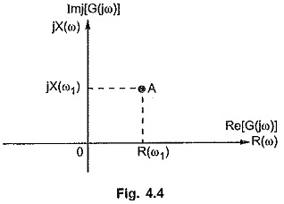
For each ω, there is separate point defined in a complex plane by the rectangular form of G(jω). For example at ω = ω1, G(jω) = R(ω1) + j X(ω1). The point can be represented as shown in the Fig. 4.4, without indication of to ω on the plane. As ω is changed, the real and imaginary parts of G(jω) get varied and define new point in a complex plane. Thus by varying ω from 0 to ∞, we can obtain the locus traced by G(jω), according to its rectangular co-ordinates.
The locus obtained by plotting the real R(ω) and imaginary X(ω) coordinates of G(jω), when ω is varied from 0 to ∞ is called complex locus. If G(jω) is an immitance function then the locus is called immitance locus of the given network. Similar to rectangular coordinates, the point can be defined in a plane by its polar coordinates. Thus varying ω from 0 to ∞ and plotting corresponding polar coordinates of G(jω), the same locus as obtained by plotting rectangular co-ordinates can be obtained. The plotting of the polar co-ordinates is shown in the Fig. 4.5. For ω = ω1, |G(jω)| at ω = ω1 is OA while ∠ G(jω) is Φ1 measured with respect to positive real axis.
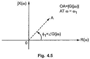
Thus as per the polar co-ordinates, each point obtained is a tip of a phasor drawn from the origin representing magnitude M, at an angle Φ measured from the positive real axis. The locus of tips of such phasors plotted for various values of ω gives the complex locus.
The locus obtained by either of these coordinate systems is always same and contains same information as contained in the magnitude and phase plots of the frequency response. The only difference is in the frequency response the variable ω has separate existence on the plot while in complex loci, the values are to be obtained by varying ω only, but ω does not have direct indication on the plots.
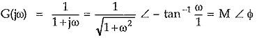
To get an idea of complex locus, let us obtained such a complex locus for the network function,
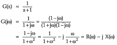
Thus preparing table of R(ω) and X(ω) values for various values of ω, we can obtain complex locus.
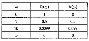
The plot is shown in the Fig. 4.6.
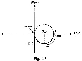
The same plot can be obtained by joining tips of the phasors defined by polar coordinates of G(jω), for same ω values.
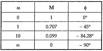
The plot is shown in the Fig. 4.7.
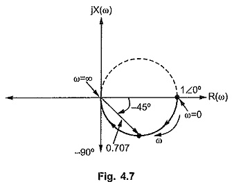
The tipper half of the circle is shown dotted which exists for negative values of ω in the range – ∞ to 0. Practically negative values of ω are nonexisting hence corresponding locus is shown dotted.
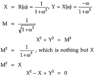
Knowing the relation between rectangular and polar coordinates and eliminating ω from the coordinates, the mathematical equation of the corresponding locus can be obtained.
In the above example,
Now complete the square
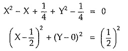
Comparing this with equation of circle,
![]()
We can conclude that this locus is a circle with center (x1,y1) i.e. (1/2,0) and the radius R = 1/2. This is as obtained in the earlier analysis.
In the various RLC networks, the impedance or admittance functions can be expressed in the polar form by substituting s = jω and tabulating M and Φ for various values of ω, the complex locus can be obtained. Similarly by identifying the loci of various parts of the circuit and combining all of them, the complete locus for the immitance function can be obtained.