Inverse Laplace Transform:
As mentioned earlier, inverse Laplace transform is calculated by partial fraction method rather than complex integration evaluation. Let F(s) is the Laplace transform of f(t) then the inverse Laplace transform is denoted as,
![]()
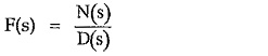
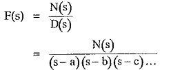
The F(s), in partial fraction method, is written in the form as,
where
N(s) = Numerator polynomial in s
D(s) = Denominator polynomial in s
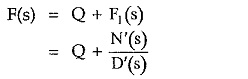
The given function F(s) can be expressed in partial fraction form only when degree of N(s) is less than D(s). Hence if degree of N(s) is equal or higher than D(s) then mathematically divide N(s) by D(s) to express F(s) in quotient and remainder form as,
where
Q = Quotient obtained by dividing N(s) by D(s)
and
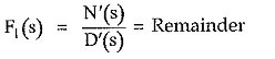
Now in the remainder, degree of N′(s) is less than D'(s) and hence F1(s) can be expressed in the partial fraction form. Once F(s) is expanded interms of partial fractions, inverse Laplace transform can be easily obtained by adjusting the terms and referring to the table of Standard Laplace transform pairs.
The roots of denominator polynomial D(s) play an important role in expanding the given F(s) into partial fractions. There are three types of roots of D(s). The method of finding partial fractions for each type is different. Let us discuss these three cases of roots of D(s).
Simple and Real Roots:
The roots of D(s) are simple and real. Hence the function F(s) can be expressed as,
where a, b, c … are the simple and real roots of D(s). The degree of N(s) should be always less than D(s). This can be further expressed as,
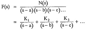
where K1, K2, K3, … are called partial fraction coefficients. The values of K1, K2, K3, … can be obtained as,
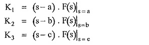
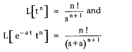
In general,
![]()
where
![]()
is standard Laplace transform pair. Hence once F(s) is expressed in terms partial fractions, with coefficients K1, K2 … Kn, the inverse Laplace transform can be easily obtained.
![]()
Multiple Roots:
The given function is of the form,
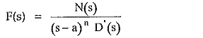
Here there is multiple root of the order ‘n’ existing at s = a. The method of writing the partial fraction expansion for such multiple roots is,
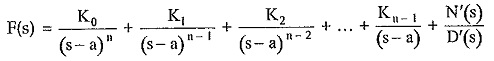
where N′(s)/D′(s) represents remaining terms of the expansion of F(s).
Here find the L.C.M. of the entire right hand side and express numerator interms of K0, K1, K2,… The numerator N(s) on left hand side is known. Compare the coefficients of all powers of s in the numerator of both sides which will give simultaneous equations interms of K0, K1, K2,… Solving these equations we can obtain the coefficients K0, K1, K2,…
For ease of solving simultaneous equations, we can find out the coefficient K0 by the same method as discussed for simple roots.
![]()
Similarly coefficients for simple roots present if any, can also be calculated by the method discussed earlier, for ease of solving simultaneous equations.
While finding Laplace inverse transform of expanded F(s) refer to standard transform pairs,
Complex Conjugate Roots:
If there exists a quadratic term in D(s) of F(s) whose roots are complex conjugates then the F(s) is expressed with a first order polynomial in s in the numerator as,
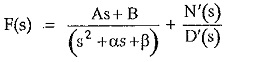
where (s2 + αs + β) is the quadratic whose roots are complex conjugates while N′(s)/D′(s) represents remaining terms of the expansion. The A and B are partial fraction coefficients.
The method of finding the coefficients in such a case is same as discussed earlier for the multiple roots. Once A and B are known then use the following method for calculating inverse Laplace transform.
Consider
![]()
Now complete the square in the denominator by calculating last term as,
![]()
where
L.T = Last term
M.T = Middle term
F.T = First term
L.T = α2/4
![]()
where![]()
Now adjust the numerator As + B in such a way that it is of the form,

Thus inverse Laplace transform of F(s) having complex conjugate roots of D(s), always contains sine, cosine or damped sine or damped cosine functions.
Inverse Laplace Transform Using Convolution Integral:
The convolution theorem states that,
![]()
Express the given F(s) as a product of two functions F1 (s) and F2 (s).
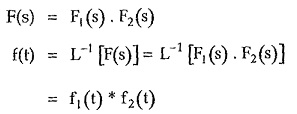
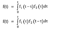
Now f1 (t) * f2 (t) is the convolution given by integral,
![]()
Thus if F(s) can be expressed as F1 (s) • F2 (s) where inverse Laplace transform of F1 (s) and F2 (s) are known as f1 (t) and f2 (t) respectively then,