Charge Simulation Method for Electric Field:
Charge Simulation Method (CSM) belongs to the family of integral methods for calculation of electric fields. There are two variations of this method: CSM with discrete charges and CSM with area charges.
Charge Simulation Method with discrete charges is based on the principle that the real surface charges on the surface of electrodes or dielectric interfaces are replaced by a system of point and line charges located outside the field domain. The position and the type of simulation charges are to be determined first and then the magnitudes of the charges are calculated so that their combined effect satisfies the boundary conditions. After determining these magnitudes by using the method of solving a system of liner equations, it is to be verified whether the systems of simulation charges fulfils the boundary conditions between the location points with sufficient accuracy. Then the voltage and field strength at any point within the field domain can be calculated analytically by the superposition of simple potential and gradient functions.
Working Principle of Charge Simulation Method:
When the conductor is excited by an applied voltage, charges appear on the surface of the conductor. These charges produce an electric field outside the conductor, while at the same time maintains the conductor at equipotential. Similarly, when a dielectric is excited by an external field, it gets polarised, i.e. the charged particles of the molecules of the dielectric get shifted from their neutral state to produce a volume of dipoles. In essence, it is possible to replace this volume polarisation by the charged surface. Charge Simulation Method employs this physical description and attempts to simulate the above-mentioned continuous charge distribution by a set of discrete charges kept just outside the computational domain. The values of these discrete charges are then evaluated by forcing the specified voltages at some selected points called contour points on the surface of the conductor and by forcing the material interface conditions at some selected points on the dielectric interface.
It is required that at any of these contour points on the electrode, the potential resulting from the superposition of the charges is equal to the electrode potential φ
Thus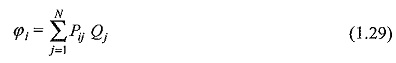
where, Pij are the potential coefficients which can be evaluated analytically for many types of charges by solving Laplace’s or Poisson’s equation. For example, in Fig. 1.5 which shows three point charges Q1, Q2 and Q3 in free space, the potential φi at point Ci will be
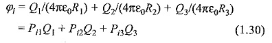
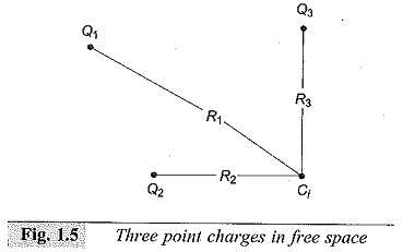
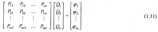
Thus, once the types of charges and their locations are defined, it is possible to relate φij and Qj quantitatively at any boundary point. In Charge Simulation Method, the simulation charges are placed outside the space where the field solution is desired (or inside any equipotential surface such as metal electrodes). If the boundary point Ci is located on the surface of a conductor, then φi at this contour point will be equal to the conductor potential φ. When this procedure is applied to m contour points, it leads to the following system of m linear equations for n unknown charges.
This equation is the basis of the CSM as discussed below.
Application of Charge Simulation Method for Single Electric Field:
If there are N conductors with known potentials in a single dielectric medium, then, for the calculation of field, the actual charges on the surfaces of these conductors are replaced by nc fictitious charges placed inside or outside the conductors. The types and positions of these charges are assumed. In order to determine their magnitudes, nb contour points are selected on the surfaces of the conductors, at known or fixed potentials and it is required that at any of these contour points the potential resulting from superposition of all the simulation charges is equal to the known conductor potential. The number of contour points is selected equal to the number of fictitious charges, i.e. n b = nc = n. Therefore, the charges are determined from
![]()
where,
- [P] = potential coefficient matrix,
- [Q] = column vector of values of unknown charges, and
- [φ] = potential of the boundary points.
After solving Eq. (1.32) to determine the magnitudes of simulation charges, it is necessary to check whether the set of calculated charges produces the actual boundary conditions everywhere on the electrode surfaces. It is possible that the potential at any point other than the contour points can be different from the actual conductor potential. Thus, Eq. (1.29) is solved at a number of check points located on the electrodes where potentials are known to determine the simulation accuracy. If simulation does not meet the accuracy, criterion, calculations are repeated by changing either the number or the location or the types of Electric Field Simulation Method and the locations of contour points.
Once adequate charge system has been determined, the potential and field at any point outside the electrodes can also be calculated:
Application of Charge Simulation Method for Multi-Dielectric Medium:
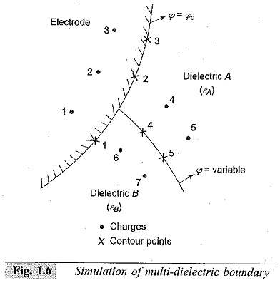
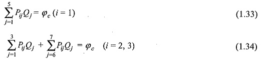
The field computations for a multi-dielectric system are more complicated than for a single dielectric. This is due to the fact that, under the influence of applied voltage, the dipoles are re-aligned in a dielectric, and this re-alignment has the effect of producing a net surface charge on the dielectric. Thus, in addition to the electrodes, each dielectric-dielectric interface needs to be simulated by the discrete charges. In the simple example of Fig. 1.6, charges 1 to 3 are used to simulate the electrode while charges 4 to 7 are used to simulate the dielectric boundary. Contour points 1 to 3 are selected on the electrode surface whereas only two contour points (i.e. 4 and 5) are selected on the dielectric boundary. In order to determine the simulation charges, a system of equations is formulated by imposing the following boundary conditions:
- at each electrode boundary, potential must be equal to the known conductor potential, and
- at each dielectric boundary, potential and normal component of the flux
density must be same, when viewed from either side of the boundary.
In formulating the equations at a given contour point, the charges which lie in the same dielectric as the contour point are ignored. For example, the potential at control point 1 is calculated by the superposition of charges 1 to 5. Similarly, the potential or field intensity at contour point 5 when viewed from the side of dielectric A will be due to the superposition of charges 1 to 3 and 6 and 7.
When the second boundary condition is applied for potential and the flux density at i = 4 to 5, the following equations are obtained:
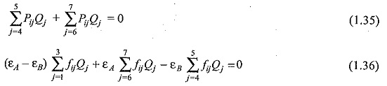
for i = 4, 5, where, fij the field coefficients in a direction which is normal to the dielectric boundary at the respective contour point. The above equations are solved to determine the unknown charges. The accuracy of Electric Field Simulation Method of multi dielectric boundaries deteriorates when the dielectric boundary has a complex profile.
The error in the Charge Simulation Method depends upon the type, number as well as the locations of the simulation charges, the locations of contour points and the complexities of the profile of the electrodes and the dielectrics.