IIR Filter Design 1-D:

In this section some practical considerations relating to the methods for the design of IIR Filter Design filters are presented. In particular, the bilinear transform is considered along with its application to the digitization of rational transfer func­tions of classical analog filters defined on the s-plane or in the framework of the wave digital filter approximation.

Review of Classical Analog Filters

Before going into the details of digitization methods, let us briefly review the main properties of the common families of analog low pass filters.

The first family of filters considered is the Butterworth filter, which consists of filter which are normally flat, that is, filters having the 2N — 1 derivative of the squared magnitude. For an Nth order filter with zero at the origin, the squared magnitude response has the form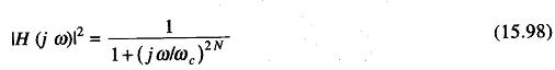

where ω_c is the cutoff frequency at which the magnitude response has an amplitude of — 3db. These filters with monotonic pass band and stop band behaviour have equally spaced poles on the s-plane, on a circle of radians.

Chebyschev filters have an equiripple behaviour, which minimises the maxi­mum error in one of the two bands, the pass band or the stop band. On the other hand in which the minimal condition is not applied, the behaviour is monotonic. The squared magnitude response is written in the form

where V_N is a Chebyschev polynomial of order N.

A third family of filters is that of elliptic filters. An elliptic filter has equiripple behaviour in both stop and pass bands. It is an optimum filter, in the sense that for a given order and given ripple specifications, it has a narrow transition band width. The squared magnitude response is given by

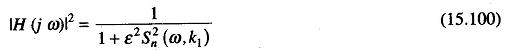
where ε is a parameter related to the pass band filter ripple equal to 1 ± 1/ (1 + ε²), where k₁ = ε/√A²-1 is a parameter related to the stop band 1/A², and S_n is the Jacobi elliptic function.

Design of Digital IIR Filters by Means of the Bilinear Transform

The poles of the filter discussed above can be easily obtained, and expressed in the form

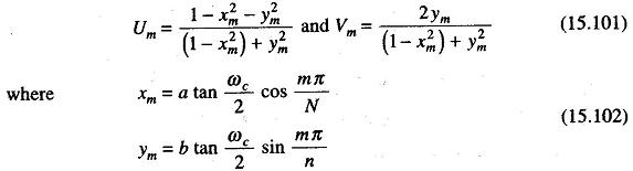
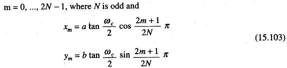
m = 0, 1, …, 2N — 1, when N is even, a and b are equal to the 1 in the Butterworth case.

Thus when the parameters of the design, N, ω_c and ε are known in the Chebyschev case, the coefficients of the filter can be obtained by computing the pole positions by means of either Eqs (15.102) or (15.103).

The problem is now to investigate the relationship between the order x of the filter N, the pass band deviation δ, and the transition bandwidth Δf, defined by the cutoff frequency f_c and the frequency f_a at which the squared magnitude frequency response is less than or equal to 1/A².

Let us now consider the three types of design specifications.

In the first case (Δf and δ fixed), the design procedure has to start with the evaluation of the order of the filter necessary to meet the specifications in terms of the desired attenuation, transition bandwidth and pass band deviation.

The pass band deviation can be controlled in the case of Chebyschev filters be ε. In any case, having defined f_c and f_a (i.e. transition bandwidth), the desired value 1/A² of |H(e^jω)|² at f_a and ε in the Chebyschev case, it is possible to determine N iteratively, starting from a first order filter and increasing the order of the filter to the point where the attenuation at f_a is greater than the desired value. At this point the design is completely determined.

In the second case (N and Δf fixed), the design is completely determined for the Butterworth filter case by obtaining the value of the attenuation at f_a directly.

In the third case (N and δ fixed), the filter is completely specified and the transition band width is directly obtainable during the design procedure.

A computer program is presented which designs Butterworth and Chebys­chev filters by means of the above relation. It also computes the coefficients of their cascade structure. The inputs to the program are the critical frequencies

f_c and f_a, the values of the desired attenuation of the filters at f_a and the value of the maximum pass band ripple if a Chebyschev filter is to be designed. The order of the filter is computed iteratively.

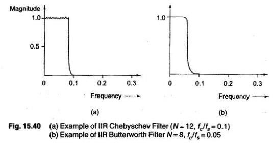
Two examples of the filter design with this program are shown in Figs 15.40 (a) and (b).

Assuming a realization structure by means of second order sections, only even order filters are designed by the program. However, it is quite simple to modify the program to design odd filters by replacing Eq. (15.102) with Eq. (15.103) and introducing a first order section in the structure.

The program presented here can be used to design only low pass filters. To design other types of filters, such as band pass, high pass and band stop, it is possible to start with the design of a normalized filter and then apply the appro­priate frequency transformation, as shown in Table 15.6. A simple routine (TRASF) to perform these transforms is presented.

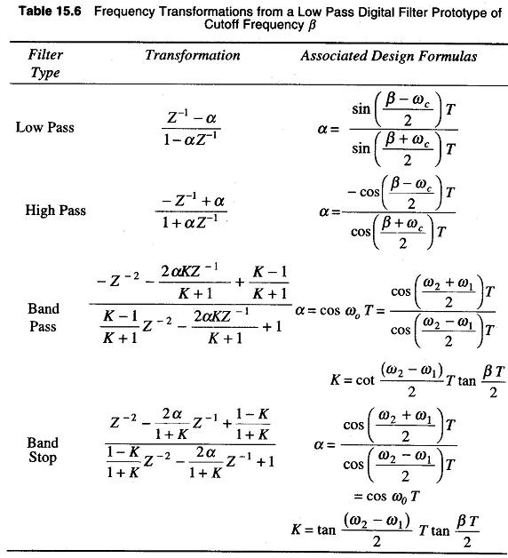
It is usually assumed that one has a low pass filter of a definite cut off frequency, say β rad/s, from which other low pass, high pass, band pass or band stop filters are required to be derived.

The low pass digital filter is said to be normalized when