Uncompensated Large Time Constants:

It is possible to compensate only one Uncompensated Large Time Constants using a PI controller. A PID controller is used to compensate for two large time constants. On technical grounds, compensation of more than two constants using a PID

Therefore if a transfer function has more than two dominant poles, only the effect of two poles can be compensated and the rest of the dominating poles do not assure desired performance.

It is therefore necessary to suggest modifications to the controller design, which takes care of this Uncompensated Large Time Constants and still provides a desired performance. This section deals with considering such Uncompensated Large Time Constants.

Before suggesting the modifications the effect of these constants on the performance may be studied in detail.

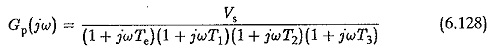
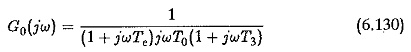
The transfer function of the plant requiring the compensation is

The controller transfer function is

Hence in the simplest case the time constant T₃ cannot the controller. The open loop transfer function of the controller is

The time constant T₃ would be the least of all the Uncompensated Large Time Constants of the plant. T_e has already been taken to be the sum of all parasitic time constants of the plant. The time constant T₃ can also be considered one such and can be added on to T_e so that the new value of T, is

with this modification the open loop transfer function is

The ratio K_e would now change to K′_e where

Substituting these relations in Eq. 6.132 we have

The value of K′_e is less than that of K_e. The effect of T₃ as a parasitic time constant adding on to T_c is to effectively decrease the ratio K_e to K′_e. The effects of decreasing the value of K_e have already been discussed. The effects due to T₃ are as follows:

1. The gain cross-over frequency increases.
2. The phase margin decreases. The damping of the system is less than the
3. The peak overshoot will be more than the desired one.

The investigation of these effects as caused by the Uncompensated Large Time Constants may be done assuming that T₃/T_e = g and jωT_e =q. The open loop transfer function given by Eq. 6.130 may be written as

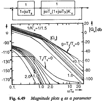
The block diagram of the system with Uncompensated Large Time Constants T₃ is shown in Fig. 6.48. The Bode plots (magnitude and phase plots) of this func­tion are shown in Fig. 6.49 for different values of g. Assuming a given value for T₀ the integration time of the controller and the controller constant, the effect of T₃ can be seen to be to decrease the phase margin. For this case the gain cross-over frequency remains the same and phase margin decreases as shown by the vertical line for different values of g(= T₃/T_e). This falls in line with the effects of change in the value of K_e to K′_e, listed above. There­fore the effect of T₃ can be considered as a change in T_e to T′_e. The value of T′_e = T_e(1 + g). Using this the open loop transfer function can be written as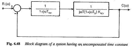

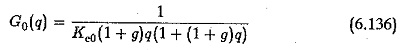
The actual transfer function given by Eq. 6.135 can be approximated by the transfer function of Eq. 6.136.

For the damping to be the same as the desired one the phase margin must be maintained at the value corresponding to q = 0. The Bode plots are drawn so that the phase and magnitude plots for q ≠ 0 are such that the phase margin is maintained at the value corresponding to g = 0. The effect of this is to shift the magnitude plots towards the left (Fig. 6.49), i.e., the gain cross-over frequency decreases. This amounts, effectively, to increasing the controller constant to maintain the value of phase margin at a reduced value of gain cross-over frequency. This can be achieved by increasing the integration time of the controller. If on the other hand the integration time does not change, the phase margin decreases causing reduced damping and increased peak overshoot. Hence the performance is poorer than the desired one.

Therefore the controller designed to compensate only two Uncompensated Large Time Constants does not give satisfactory performance. To get the desired performance its design must be modified. The above discussion gives the direction in which the modification may be oriented. As the damping is decided by the phase margin, the various constants of the controller must be chosen such that phase margin does not change when T₃ is taken into consideration. This can be ea­sily achieved by introducing a correction by which the phase of the function changes bringing the phase margin to the desired value. Using this factor the open loop transfer function of Eq. 6.136 is given by

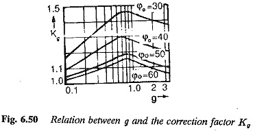
It is equivalent to changing to the value of gain cross-over frequency to 1/(K_gK_e0(1+g)). The value of K_g can be chosen such that the magnitude and phase plots for the value of g are such that the phase margin of the transfer function is same as that of the transfer function for g = 0. A relation can be derived between g and K_g to achieve the desired phase margin. Typical curves are shown in Fig. 6.50 with the phase margin as a parameter. This is equivalent to changing the integration time of the controller. The gain cross-over changes to 1/(K_g(1+g)K_e0)..

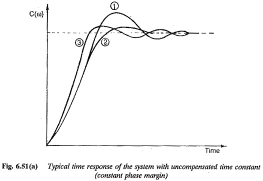
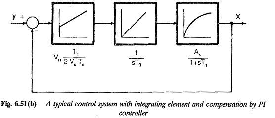
Typical time responses of the system are shown in Fig. 6.51. Curve 1 indi­cates the time response of the system with its Uncompensated Large Time Constants. This shows a characteristic increase in peak overshoot due to T₃. Curve 2 indicates the time response of the system with the correction factor. Curve 3 indicates the desired time response, or time response with T₃ = 0. A close examination shows that the correction introduced improves the performance so that the peak overshoot is within the desired value. This is because the phase margin decides the damping and the overshoot very much and it is maintained constant by a proper correction. However the rise time changes. Therefore, while designing a controller for a system having three time con­stants of which two can be directly compensated, the integration time should be properly chosen so that the effect of the third time constant is minimal. The integration time of the controller is

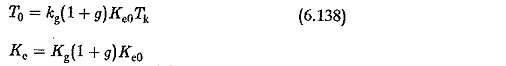
The value of K_g can be read from Fig. 6.50.