Gauss Seidel Method | Flow chart

Gauss Seidel Method:

The Gauss Seidel Method (GS) is an iterative algorithm for solving a set of non-linear algebraic equations. To start with, a solution vector is assumed, based on guidance from practical experience in a physical situation. One of the equations is then used to obtain the revised value of a particular variable by substituting in it the present values of the remaining variables. The solution vector is immediately updated in respect of this variable. The process is then repeated for all the variables thereby completing one iteration. The iterative process is then repeated till the solution vector converges within prescribed accuracy. The convergence is quite sensitive to the starting values assumed. Fortunately, in a load flow study a starting vector close to the final solution can be easily identified with previous experience.

To explain how the Gauss Seidel Method is applied to obtain the load flow solution, let it be assumed that all buses other than the slack bus are PQ buses. We shall see later that the method can be easily adopted to include PV buses as well. The slack bus voltage being specified, there are (n – 1) bus voltages starting values of whose magnitudes and angles are assumed. These values are then updated through an iterative process. During the course of any iteration, the revised voltage at the ith bus is obtained as follows:

From Eq. (6.5)

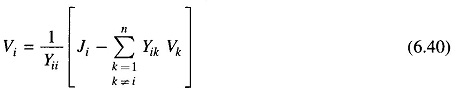
Substituting for J_i from Eq. (6.39) into (6.40)

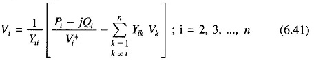
The voltages substituted in the right hand side of Eq. (6.41) are the most recently calculated (updated) values for the corresponding buses. During each iteration voltages at buses i = 2, 3, …, n are sequentially updated through use of Eq. (6.41). V₁, the slack bus voltage being fixed is not required to be updated. Iterations are repeated till no bus voltage magnitude changes by more than a prescribed value during an iteration. The computation process is then said to converge to a solution.

If instead of updating voltages at every step of an iteration, updating is carried out at the end of a complete iteration, the process is known as the Gauss iterative method. It is much slower to converge and may sometimes fail to do so.

Algorithm for Load Flow Solution:

Presently we shall continue to consider the case where all buses other than the slack are PQ buses. The steps of a computational algorithm are given below:

With the load profile known at each bus (i.e. P_Di and Q_Diknown), allocate P_Gi and Q_Gi to all generating stations. While active and reactive generations are allocated to the slack bus, these are permitted to vary during iterative computation. This is necessary as voltage magnitude and angle are specified at this bus (only two variables can be specified at any bus). With this step, bus injections (P_i+ jQ_i) are known at all buses other than the slack bus.
Assembly of bus admittance matrix Y_BUS: With the line and shunt admittance data stored in the computer, Y_BUS is assembled by using the rule for self and mutual admittances. Alternatively Y_BUS is assembled using Eq. (6.23) where input data are in the form of primitive matrix Y and singular connection matrix A.
Iterative computation of bus voltages (V_i; i = 2, 3,…, n): To start the iterations a set of initial voltage values is assumed. Since, in a power system the voltage spread is not too wide, it is normal practice to use a flat voltage start, e. initially all voltages are set equal to (1 + j0) except the voltage of the slack bus which is fixed. It should be noted that (n – 1) equations (6.41) in complex numbers are to be solved iteratively for finding (n – 1) complex voltages V₂, V₃, …, V_n. If complex number operations are not available in a computer, Eqs (6.41) can be converted into 2(n – 1) equations in real unknowns (e_i, f_i or |V_i|, δ_i) by writing

A significant reduction in the computer time can be achieved by performing in advance all the arithmetic operations that do not change with the iterations.

Define

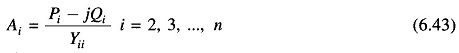
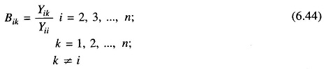
Now for the (r + 1)th iteration, the voltage Eq. (6.41) becomes

The iterative process is continued till the change in magnitude of bus voltage, |ΔV_i^(r+1)|, between two consecutive iterations is less than a certain tolerance for all bus voltages, i.e.

Computation of slack bus power: Substitution of all bus voltages computed in step 3 along with V₁ in Eq. (6.25b) yields S₁^* = P₁ – jQ₁.
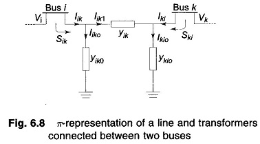
Computation of line flows: This is the last step in the load flow analysis wherein the power flows on the various lines of the network are computed. Consider the line connecting buses i and k. The line and transformers at each end can be represented by a circuit with series admittance y_ik and two shunt admittances y_ik0 and y_ki0 as shown in Fig. 6.8.

The current fed by bus i into the line can be expressed as

The power fed into the line from bus i is.

Similarly, the power fed into the line from bus k is

The power loss in the (i – k)th line is the sum of the power flows determined from Eqs. (6.48) and (6.49). Total transmission loss can be computed by summing all the line flows (i.e. S_ik + S_ki for all i, k).

It may be noted that the slack bus power can also be found by summing the flows on the lines terminating at the slack bus.

Acceleration of convergence:

Convergence in the Gauss Seidel Method can sometimes be speeded up by the use of the acceleration factor. For the ith bus, the accelerated value of voltage at the (r + 1)th iteration is given by

where α is a real number called the acceleration factor. A suitable value of α for any system can be obtained by trial load flow studies. A generally recommended value is α = 1.6. A wrong choice of cc may indeed slow down convergence or even cause the method to diverge.

This concludes the load flow analysis for the case of PQ buses only.

Algorithm Modification when PV Buses are also Present:

At the PV buses, P and |V| are specified and Q and δ are the unknowns to be determined. Therefore, the values of Q and δ are to be updated in every Gauss Seidel Method iteration through appropriate bus equations. This is accomplished in the following steps for the ith PV bus.

From Eq. (6.26b)

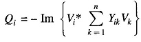
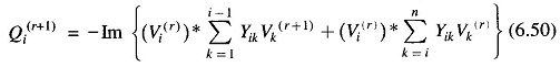
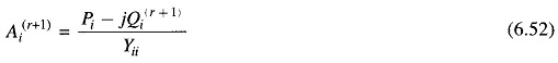
The revised value of Q_i is obtained from the above equation by substituting most updated values of voltages on the right hand side. In fact, for the (r + 1)th iteration one can write from the above equation

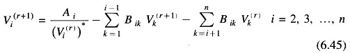
The revised value of δ_i is obtained from Eq. (6.45) immediately following step 1. Thus

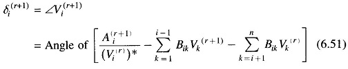
where

The algorithm for PQ buses remains unchanged.

As explained already, physical limitations of Q generation require that Q demand at any bus must be in the range Q_min→Q_max. If at any stage during the computation, Q at any bus goes outside these limits, it is fixed at Q_min or Q_max as the case may be, and the bus voltage specification is dropped, i.e. the bus is now treated like a PQ bus. Thus step 1 above branches out to step 3 below.

_3.If Q_i^(r+1) < Q_i,min_, set Q_i^(r+1) = Q_i,min and treat bus i as a PQ bus. Compute A_i^(r+1) and V_i^(r+1) from Eqs. (6.52) and (6.45), respectively. If Q_i^(r+1) > Q_i,_max, set Q_i^(r+1) = Qi,_max and treat bus i as a PQ bus. Compute A_i^(r+1) and V_i^(r+1) from Eqs. (6.52) and (6.45), respectively.

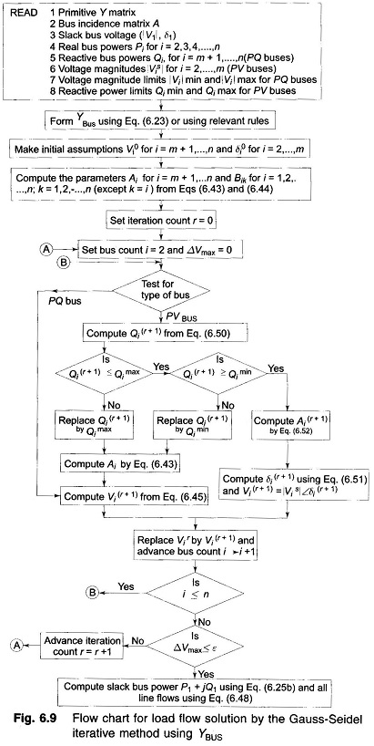
Now all the computational steps are summarized in the detailed flow chart of Fig. 6.9 which serves as a basis for the reader to write his own computer programme. It is assumed that out of n buses, the first is slack as usual, then 2, 3, …, m are PV buses and the remaining m + 1, n are PQ buses.