Formation of YBUS By Singular Transformation:

Formation of YBUS By Singular Transformation – The matrix pair Y_BUS and Z_BUS form the network models for load flow studies. The Y_BUS can be alternatively assembled by use of singular transformations given by a graph theoretical approach. This alternative approach is of great theoretical and practical significance and is therefore discussed here.

To start with, the graph theory is briefly reviewed.

Graph Theory:

To describe the geometrical features of a network, it is replaced by single line segments called elements whose terminals are called nodes. A linear graph depicts .the geometrical interconnection of the elements of a network. A graph is connected if, and only if, there is a path between every pair of nodes. If each element of a connected graph is assigned a direction, it is called an oriented graph.

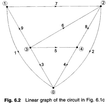
Power networks are so structured that out of the m total nodes, one node (normally described by 0) is always at ground potential and the remaining n = m – 1 nodes are the buses at which the source power is injected. Figure 6.2 shows the graph of the power network of Fig. 6.1c.

It may be noted here that each source and the shunt admittance connected across it are represented by a single element. In fact, this combination represents the most general network element and is described under the subheading “Primitive Network”.

A connected subgraph containing all the nodes of a graph but having no closed paths is called a tree. The elements of a tree are called branches or tree branches. The number of branches b that form a tree are given by

Those elements of the graph that are not included in the tree are called links (or link branches) and they form a subgraph, not necessarily connected, called cotree. The number of links l of a connected graph with e elements is

Note that a tree (and therefore, cotree) of a graph is not unique.

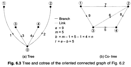
A tree and the corresponding cotree of the graph of Fig. 6.2 are shown in Fig. 6.3. The reader should try and find some other tree and cotree pairs.

If a link is added to the tree, the corresponding graph contains one closed path called a loop. Thus a graph has as many loops as the number of links.

Primitive Network:

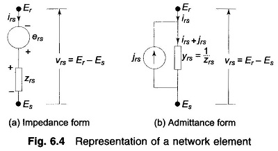
A network element may in general contain active and passive components. Figures 6.4a and b show, respectively, the alternative impedance and admittance form representation of a general network element. The impedance form is a voltage source e_rs in series with an impedance z_rs; while the admittance form is a current source j_rs in parallel with an admittance y_rs. The element current is i_rs and the element voltage is

where E_r and E_s are the voltages of the element nodes r and s, respectively.

It may be remembered here that for steady state AC performance, all element variables (ν_rs, E_r, E_s, i_rs, j_rs) are phasors and element parameters (z_rs, y_rs) are complex numbers.

The voltage relation for Fig. 6.4a can be written as

Similarly, the current relation for Fig. 6.4b is

The forms of Figs. 6.4a and b are equivalent wherein the parallel source current in admittance form is related to the series voltage in impedance form by

Also

A set of unconnected elements is defined as a primitive network. The performance equations of a primitive network are given below:

In impedance form

In admittance form

Here V and I are the element voltage and current vectors respectively, and J and E are the source vectors. Z and Y are referred to as the primitive impedance and admittance matrices, respectively. These are related as Z = Y ^-1. If there is no mutual coupling between elements, Z and Y are diagonal where the diagonal entries are the impedances/admittances of the network elements and are reciprocal.

Network Variables in Bus Frame of Reference:

Linear network graph helps in the systematic assembly of a network model. The main problem in deriving mathematical models for large and complex power networks is to select a minimum or zero redundancy (linearly independent) set of current or voltage variables which is sufficient to give the information about all element voltages and currents. One set of such variables is the b tree voltages. It may easily be seen by using topological reasoning that these variables constitute a non-redundant set. The knowledge of b tree voltages allows us to compute all element voltages and therefore, all bus currents assuming all element admittances being known.

Consider a tree graph shown in Fig. 6.3a where the ground node is chosen as the reference node. This is the most appropriate tree choice for a power network. With this choice, the b tree branch voltages become identical with the bus voltages as the tree branches are incident to the ground node.

Bus Incidence Matrix:

For the specific system of Fig. 6.3a, we obtain the following relations between the nine element voltages and the four bus (i.e. tree branch) voltages V₁, V₂, V₃ and V₄.

or, in matrix form

where the bus incidence matrix A is

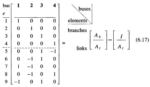
This matrix is rectangular and therefore singular. Its elements a_ik are found as per the following rules:

a_ik =1 if ith element is incident to and oriented away from the kth node (bus)

= – 1 if ith element is incident to but oriented towards the kth node

= 0 if the ith element is not incident to the kth node

Substituting Eq. (6.16) into Eq. (6.14), we get

Pre multiplying by A^T,

Each component of the n-dimensional vector A^TI is the algebraic sum of the element currents leaving the nodes 1, 2, …, n.

Therefore, the application of the KCL must result in

Similarly, each component of the vector A^TJ can be recognized as the algebraic sum of all source currents injected into nodes 1, 2, …, n. These components are therefore the bus currents . Hence we can write

Equation (6.19) then is simplified to

Thus, following an alternative systematic approach, we have in fact, obtained the same nodal current equation as (6.6). The bus admittance matrix can then be obtained from the formation of YBUS by singular transformation of the primitive Y, i.e.

A computer programme can be developed to write the bus incidence matrix A from the interconnection data of the directed elements of the power system. Standard matrix transpose and multiplication subroutines can then be used to compute Y_BUS from Eq. (6.23).