Time and Energy Loss in Transient Operations:
Starting, braking, speed change and speed reversal are transient operations. Time and Energy Loss in Transient Operations can be evaluated by solving Eq. (2.19) along with motor circuit equations.![]()
When T and TL are constants or proportionals to speed, Eq. (2.19) will be a first order linear differential equation. Then it can be solved analytically. When T or TL is neither constant nor proportional to speed, (2.19) will be a non-linear differential equation. It could then be solved numerically by Runga-Kutta method.
For any of the above mentioned transients, final speed is an equilibrium speed. Theoretically, transients are over in infinite time, which is not so in practice. In order to resolve this anomaly, Time and Energy Loss in Transient Operations is considered to be over when 95% change in speed has taken place. For example, when speed changes from ωm1 to equilibrium speed ωme, time taken for the speed to change from ωm1 to [ωm1 + 0.95(ωme – ωm1)] is considered to be equal to the transient time.
Transient time and energy loss can also be computed with satisfactory accuracy using steady-state speed-torque and speed-current curves of motor and speed-torque curve of load. This is because mechanical time constant of a drive is usually very large compared to electrical time constant of motor. Consequently, electrical transients die down very fast and motor operation can be considered to take place along the steady-state speed-torque and speed-current curves.
From Eq. (2.2)
![]()
where T(ωm) and Tl(ωm) indicate that the motor and load torques are functions of drive speed ωm. Time taken for drive speed to change from ωm1 to ωm2 is obtained by integrating Eq. (2.21)
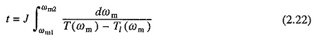
Equation (2.22) can be integrated only if functions T(ωm) and Tl(ωm) are known and are of integral form. Otherwise the integral is evaluated graphically. Expression on the right of Eq. (2.22) is the area between the reciprocal of the acceleration { J/[T(ωm) – Tl(ωm)]} VS ωm curve and ωm axis (Fig. 2.8). The transient time can be evaluated by measuring this area.
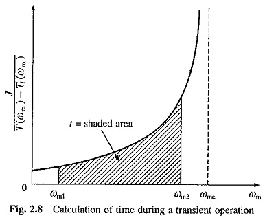
When ωm2 is an equilibrium speed ωme, then the reciprocal of acceleration will become infinite at ωme. Consequently, time evaluated this way will be infinite. Therefore, in this case transient time is computed by measuring the area between speeds ωm1 and ωm1 + 0.95(ωm2 – ωm1).
Energy dissipated in a motor winding during a transient operation is given by
where R is the motor winding resistance and i is the current flowing through it.
In many applications, by making use, of speed-torque expressions for motor and load, it is possible to arrange Eq. (2.23) in integrable form. However, this is not possible in applications where nonlinear impedance is present in the motor circuit. Then Eq. (2.23) is evaluated graphically using steady-state speed-torque and speed-current curves, as:
By graphical solution of Eq. (2.22), ωm vs t curve is obtained. From this curve and steady-state speed-current curve, i2 vs t curve is obtained. Area enclosed between this curve and time axis multiplied by R gives the energy dissipated in motor winding. This approach can also handle nonlinear resistance R, which varies as a function of i. Here i2R vs time curve is plotted. Area between this curve and the time axis gives the energy dissipated.