Radar Performance Factors:
Quite apart from being limited by the curvature of the earth, the maximum range of a radar Set depends on a number of other Radar Performance Factors. These can now be discussed, beginning with the classical radar range equation.
Radar Range Equation:
To determine the maximum range of a radar set, it is necessary to determine the power of the received echoes, and to compare it with the minimum power that the receiver can handle and display satisfactorily. If the transmitted pulsed power is Pt (peak value) and the antenna is isotropic, then the power density at a distance r from the antenna will be given by
![]()
However, antennas used in radar are directional, rather than isotropic. If Ap is the maximum power gain of the antenna used for transmission, so the power density at the target will be

The power intercepted by the target depends on its Radar Cross Section, or effective area. If this area is S, the power impinging on the target will be
![]()
The target is not an antenna. Its radiation may be thought of as being omnidirectional. The power density of its radiation at the receiving antenna will be

Like the target, the receiving antenna intercepts a portion of the reradiated power, which is proportional to the cross-sectional area of the receiving antenna. However, it is the capture area of the receiving antenna that is used here. The received power is

where
Ao = capture area of the receiving antenna,
If (as is usually the case) the same antenna is used for both reception and transmission, The maximum power gain is given by![]()
Substituting Equation (16-11) into (16-10) gives
![]()
The maximum range rmax will be obtained when the received power is equal to the minimum receivable power of the receiver, Pmin. Substituting this into Equation (16-12), and making r the subject of the equation, we have
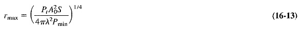
Alternatively, if Equation (16-11) is turned around so that Ao=Apλ2/4π is substituted into Equation (16-13), we have

Equations (16-13) and (16-13a) represent two convenient forms of the radar range equation, simplified to the extent that the minimum receivable power Pmin has not yet been defined. It should also be pointed out that idealized conditions have been employed. Since neither the effects Of the ground nor other absorption and interference have been taken into account, the maximum range in practice is often less than that indicated by the radar range equation.
Factors influencing maximum range:
A number of very significant and interesting conclusions may be made if the radar range equation is examined carefully. The first and Most obvious is that the maximum range is proportional to the fourth root of the peak transmitted pulse power. The peak power must be increased sixteenfold, all else being constant, if a given maximum range is to be doubled. Eventually, such a power increase obviously becomes uneconomical in any particular Radar Performance Factors system.
Equally obviously, a decrease in the minimum receivable power will have the same effect as raising the transmitting power and is thus a very attractive alternative to it. However, a number of other factors are involved here. Since Pmin is governed by the sensitivity of the receiver (which in turn depends on the noise figure), the minimum receivable power may be reduced by a gain increase of the receiver, accompanied by a reduction in the noise at its input. Unfortunately, this may make the receiver more susceptible to jamming and interference, because it now relies more on its ability to amplify weak signals (which could include the interference), and less on the sheer power of the transmitted and received pulses. In practice, some optimum between transmitted power and minimum received power must always be reached.
The reason that the range is inversely proportional to the fourth power of the transmitted peak power is simply that the signals are subjected twice to the operation of the inverse square law, once on the outward journey and once on the return trip. By the same token, any property of the Radar Performance Factors system that is used twice, i.e., for both reception and transmission, will show a double benefit if it is improved. Equation (16-13) shows that the maximum range is proportional to the square root of the capture area of the antenna, and is therefore directly proportional to its diameter if the wavelength remains constant. It is thus apparent that possibly the most effective means of doubling a given maximum radar system range is to double the effective diameter of the antenna. This is equivalent to doubling its real diameter if a parabolic reflector is used. Alternatively, a reduction in the wavelength used, i.e., an increase in the frequency, is almost as effective. There is a limit here also. As we know, the beamwidth of an antenna is proportional to the ratio of the wavelength to the diameter of the antenna. Consequently, any increase in the diameter-to-wavelength ratio will reduce the beamwidth. This is very useful in some radar applications, in which good discrimination between adjoining targets is required, but it is a disadvantage in some search radars. It is their function to sweep a certain portion of the sky, which will naturally take longer as the beamwidth of the antenna is reduced.
Finally, Equation (16-13) shows that the maximum radar range depends on the target area, as might be expected. Also, ground interference will limit this range. The presence of a conducting ground, it will be recalled, has the effect of creating an interference pattern such that the lowest lobe of the antenna is some degrees above the horizontal. A distant target may thus be situated in one of the interference zones, and will therefore not be sighted until it is quite close to the radar set. This explains the development and emphasis of “ground-hopping” military air-craft, which are able to fly fast and close to the ground and thus remain undetectable for most of their journey.
Effects of Noise:
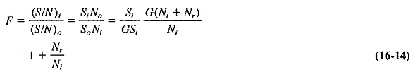
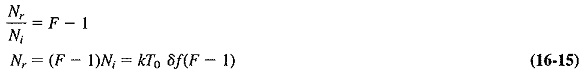
The previous section showed that noise affects the maximum Radar Performance Factors range insofar as it determines the minimum power that the receiver can handle. The extent of this can now be calculated exactly. From the definition of noise figure, it is possible to calculate the equivalent noise power generated at the input of the receiver, Nr. This is the power required at the input of an ideal receiver having the same noise figure as the practical receiver. We then have
where
Si = input signal power
Ni = input noise power
So = output signal power
No = output noise power
G = power gain of the receiver
We have
where
kTo δf = noise input power of receiver
k = Boltmann’s constant = 1.38 X 10⁻²³ J/K
T0 = standard ambient temperature = 17°C = 290 K
δf = bandwidth of receiver
It has been assumed that the antenna temperature is equal to the standard ambient temperature, which may or may not be true, but the actual antenna temperature is of importance only if a very low-noise amplifier is used.
The minimum receivable signal for the receiver, under so-called threshold detection conditions, is equal to the equivalent noise power at the input of the receiver, as just obtained in Equation (16-15). This may seem a little harsh, especially since much higher ratios of signal to noise are used in continuous modulation systems. However, it must be realized that the echoes from the target are repetitive, whereas noise impulses are random. An integrating procedure thus takes place in the receiver, and meaningful echo pulses may be obtained although their amplitude is no greater than that of the noise impulses. This may be understood by considering briefly the display of the received pulses on the cathode-ray tube screen. The signal pulses will keep recurring at the same spot if the target is stationary, so that the brightness at this point of the screen is maintained (whereas the impulses due to noise are quite random and therefore not additive). If the target itself is in rapid motion, i.e., moves significantly between successive scans, a system of moving-target indication may be used. Substituting these findings into Equation (16-13), we have
![]()
Equation (16-16) is reasonably accurate in predicting maximum range, provided that a number of factors are taken into account when it is used. Among these are system losses, antenna imperfection, receiver nonlinearities, anomalous propagation, proximity of other noise sources (including deliberate jamming) and operator errors and/or fatigue (if there is an operator). It would be safe to call the result obtained with the aid of this equation the Maximum Theoretical Range, and to realize that the maximum practical range varies between 10 and 100 percent of this value. However, range is sometimes capable of exceeding the theoretical maximum under unusual propagating conditions, such as superrefraction.
It is possible to simplify Equation (16-16), which is rather cumbersome as it stands. Substituting for the capture area in terms of the antenna diameter (A0=0.65πD2/4) and for the various constants, and expressing the maximum range in kilometers, allows simplification to

where
rmax = maximum radar range, km
Pt = peak pulse power, W
D = antenna diameter, m
S = effective cross-sectional area of target, m2
δf = receiver bandwidth, Hz
A = wavelength, m
F = noise figure (expressed as a ratio)
Target Properties:
In connection with the derivation of the radar range equation, a quantity was used but not defined. This was the radar cross section, or effective area, of the target. For targets whose dimensions are large compared to the wavelength, as for aircraft microwave Radar Performance Factors is used, the radar cross section may be defined as the projected area of a perfectly conducting sphere which would reflect the same power as the actual target reflects, if it were located at the same spot as the target. The practical situation is far from simple.
First of all, the radar cross section depends on the frequency used. If this is such that the target is small compared to a wavelength, its cross-sectional area for Radar Performance Factors appears much smaller than its real cross section. Such a situation is referred to as the Rayleigh region. When the circumference of a spherical target is between 1 and 10 wavelengths, the radar cross section oscillates about the real one. This is the so-called resonance region. Finally, for shorter wavelengths (in the optical region) the radar and true cross sections are equal.
Quite apart from variations with frequency, the radar cross section of a target will depend on the polarization of the incident wave, the degree of surface roughness (if it is severe), the use of special coatings on the target and, most importantly of all, the aspect of the target. For instance, a large jet aircraft, measured at 425 MHz, has been found to have a radar cross section varying between 0.2 and 300 m2 for the fuselage, depending on the angle at which the radar pulses arrived on it. The situation is seen to be complex because of the large number of factors involved, so that a lot of the work is empirical.