Practical Differentiator:

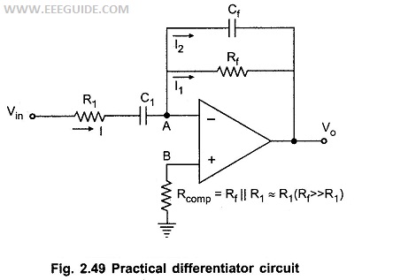
The noise and stability at high frequency can be corrected, in the practical differentiator circuit using the resistance R₁ in series with C₁ and the capacitor C_f in parallel with resistance R_f.

The circuit is shown in the Fig. 2.49. The resistance R_comp is used for bias compensation.

Analysis of the Practical Differentiator:

As the input current of op-amp is zero, there is no current input at node B. Hence it is at the ground potential. From the concept of the virtual ground, node A is also at the ground potential and hence V_B = V_A = 0V.

For the current I, we can write

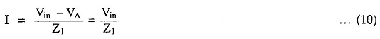
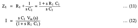
where Z₁ = R₁ in series with C₁

So in Laplace domain we can write,

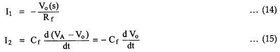
Now the current I₁ is,

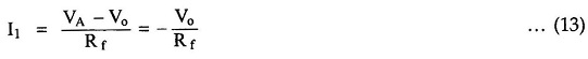
In Laplace,

Taking we get,

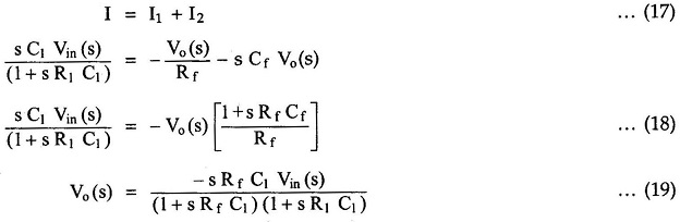
Applying at node A,

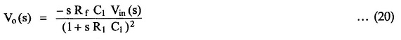
If R_fC_f = R₁C₁ then

The time constant R_fC₁ is much greater than R₁C₁ or R_fC_f and hence the equation (20) reduces to,

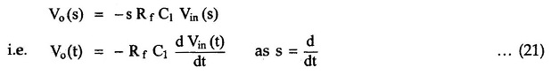
Thus the output voltage is the R_fC₁ times the differentiation of the input.

It may be noted that though R_fC₁ is much larger than R_fC_f or R₁C₁, it is less than or equal to the time period T of the input, for the true differentiation.

Applications of Practical Differentiator:

The practical differentiator circuits are most commonly used in :

1. In the wave shaping circuits to detect the high frequency components in the input signal.
2. As a rite-of-change detector in the FM demodulators.
3. The differentiator circuit is avoided in the analog computers.