Heating and Cooling Curves of Electrical Drives:

An accurate prediction of Heating and Cooling Curves of Electrical Drives rise inside an electrical motor is very difficult owing to complex geometrical shapes and use of heterogeneous materials. Since conductivities of various materials do not differ by a large amount, a simple thermal model of the machine can be obtained by assuming machine to be a homogeneous body. Although inaccurate, such a model is good enough for a drive engineer whose job is only to select the motor rating for a given application ensuring that temperatures in various parts of motor body do not exceed the safe limits.

Let the machine, which is assumed to be a homogeneous body, and the cooling medium has following parameters at time t:

P₁ = Heat developed, joules/sec or watts.

P₂ = Heat dissipated to the cooling medium, joules/sec or watts.

W = Weight of the active parts of machine, kg.

h = Specific heat, Joules per kg per °C.

A = Cooling surface, m².

d = Coefficient of heat transfer or specific heat dissipation, joules/sec/m²/°C.

θ = Mean temperature rise, °C.

During a time increment dt, let the machine temperature rise be dθ. Since,

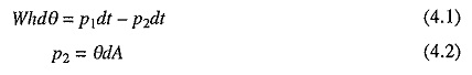
Substituting in Eq. (4.1) and rearranging the terms

C is the thermal capacity of the machine, watts/°C, and D the heat dissipation constant, watts/°C. Heat dissipation mainly occurs through convection. Typical values of d are in the range of 40 of 600 W/m²/°C. The first order differential equation (4.3) has a solution

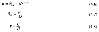
Constant of integration K is obtained by substituting the temperature rise at t = 0 in Eq. (4.6). When the initial temperature rise is θ₁, Eq. (4.6) has a solution

τ, which has the dimension of time, is known as the heating (or thermal) time constant of the machine. In Eq. (4.9) as t = ∞, θ = θ_ss. Thus θ_ss is the steady state temperature of the machine when it is continuously heated by power P₁. At this temperature, all the heat produced in machine is dissipated to the surrounding medium.

Let the load on machine be thrown off after its temperature rise reaches a value θ₂. Heat loss will reduce to a small value P′₁ and cooling operation of the motor will^–begin. Let the new value of heat dissipation constant be D′. If time is measured from the instant the load is thrown off, then

Solving this first order differential equation subjected to the initial condition, θ = θ₂ at t = 0, gives

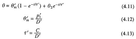
θ′_ss is again steady state temperature rise for new conditions of operation and τ′ is known as the Cooling (or thermal) Time Constant of the machine.

If motor were disconnected from the supply during Heating and Cooling Curves of Electrical Drives then P′₁ = θ′_ss = 0, suggesting that the final temperature attained by the motor will be ambient temperature. Substituting in Eq. (4.11) gives

Eqs. (4.9) and (4.14) suggest that both heating time constant τ and cooling time constant τ′ depend on the respective heat dissipation constants D and D′, which in turn depend on the velocity of cooling air.

In self cooled motors, where cooling fan is mounted on motor shaft, the velocity of cooling air varies with motor speed, thus varying cooling time constant τ′. Cooling time constant at standstill is much larger than when running. Therefore, in high performance, and medium and high power variable speed drives, motor is always provided with separate forced cooling, so that motor cooling be independent of speed.

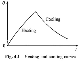
Figure 4.1 shows the variation of motor temperature rise with time during Heating and Cooling Curves of Electrical Drives. Thermal time constants of a motor are far larger than electrical and mechanical time constants. While electrical and mechanical time constants have a typical ranges of 1 to 100 ms and 10 ms to 10 s, the thermal time constants may vary from 10 min to couple of hours.