Electric Field Equation:
Electric Field Equation – In recent years, several numerical methods for solving partial differential equations which include Laplace’s and Poisson’s equations have become available. There are inherent difficulties in solving these equations for two or three dimensional fields with complex boundary conditions, or for insulating materials with different permittivities and/or conductivities.
Proper design of any high voltage apparatus requires a complete knowledge of the electric field distribution. For a simple physical system with some symmetry, it is possible to find an analytical solution. However, in many cases, the physical systems are very complex and therefore in such cases, numerical methods are employed for the calculation of electric fields. Essentially, four types of numerical methods are commonly employed in high voltage engineering applications. They are: Finite Difference Method (FDM), Finite Element Method (FEM), Charge Simulation Method (CSM) and Surface Charge Simulation Method (SSM) or Boundary Element Method (BEM). The first two methods are generally classified as domain methods and the last two are categorized as boundary methods.
The principal task in the computation of Electric Field Equation is to solve the Poisson’s equation Eq. (1.10). In case of space charge-free fields the equation reduces to Laplace’s equation Eq. (1.1 1). Personal computers have the required computational power to solve these problems. However, computing times and the amount of memory to achieve the desired accuracy still play a dominant role. Further, another important aspect for the acceptance of a method is the ease with which it can be used to describe the problem. A brief description of each of these methods is given in the following sections.
Finite Difference Method (FDM)
Apart from other numerical methods for solving partial differential equations, the Finite Difference Method (FDM) is universally applied to solve linear and even non-linear problems. Although the applicability of difference equations to solve the Laplace’s equation was used earlier, it was not until 1940s that FDMs have been widely used. The applicability of FDMs to solve general partial differential equation is well documented in specialised books.
The field problem for which the Laplace’s or Poisson’s equation applies is given within a (say x, y), plane, the area of which is limited by given boundary conditions, i.e. by contours on which some field quantities are known. Every potential φ and its distribution within the area under consideration will be continuous. Therefore, an unlimited number of φ (x, y) values will be necessary to describe the complete potential distribution. Since any numerical computation can provide only a limited amount of information, discretization of the area will be necessary to represent all the nodes for which the solution is needed. Such nodes are generally produced by any net or grid laid down on the area’ as shown in Fig. 1.2.
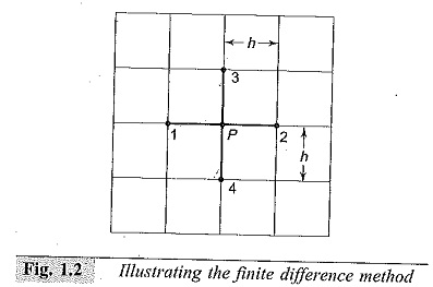
The unknown potential φ (p) can be expressed by the surrounding potentials which are assumed to be known for the single difference equation. For every two-dimensional problem, most of the field region can be subdivided by a regular square net. Then, if the step size chosen for discretization is h, the following approximate equation becomes valid.
![]()
In the above equation, φ1 + φ2 + φ3 + φ4 are the potentials at the immediate neighbourhood nodes with respect to the node p of interest (of which the potential φ(p) needs to be determined). The potentials at the neighbourhood points are expected to be known a priori, either from given boundary conditions or from any previous computational results. The term F(p) arises if the field region is governed by the Poisson’s equation, (i.e. the relation ∇2φ=F(p) holds good).
Thus, any general field problem to be treated needs sub-division of the finite plane by a predominantly regular grid, which is supplemented by irregular elements at the boundaries, if required. The whole grid will then contain n nodes, for which the potential φ(p) is to be calculated. Then, a system of n simultaneous equations would result. Here, it may be noted that simple problems with small number of unknowns can be treated by long hand computation using the concept of residuals and point relaxation. For more complex problems, machine computation is necessary and iterative schemes are most efficient in combination with successive relaxation methods.
Finite Element Method (FEM)
Finite Element Method is widely used in the numerical solution of Electric Field Equation, and became very popular. In contrast to other numerical methods, FEM is a very general method and therefore is a versatile tool for solving wide range of Electric Field Equation.
The finite element analysis of any problem involves basically four steps:
(a)Finite Element Discretization
To start with, the whole problem domain is ficticiously divided into small areas/ volumes called elements (see Fig. 1.3). The potential, which is unknown throughout the problem domain, is approximated in each of these elements in terms of the potential at their vertices called nodes. As a result of this the potential function will be unknown only at the nodes. Normally, a certain class of polynomials, is used for the interpolation of the potential inside each element in terms of their nodal values. The coefficients of this interpolation function are then expressed in terms of the unknown nodal potentials. As a result of this, the interpolation can be directly carried out in terms of the nodal values. The associated algebraic functions are called shape frictions. The elements derive their names through their shape, i.e. bar elements in one dimension (1D), triangular and quadrilateral elements in 2D, and tetrahedron and hexahedron elements for 3D problems.
(b)Governing Equations
The potential Ve within an element is first approximated and then interrelated to the potential distributions in various elements such that the potential is continuous across inter-element boundaries. The approximate solution for the whole region then becomes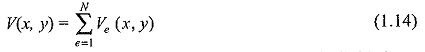
where N is the number of elements into which the solution region is divided. The most common form of approximation for the voltage V within an element is a polynomial approximation
![]()
For the triangular element, and for the quadrilateral element the equation becomes
![]()
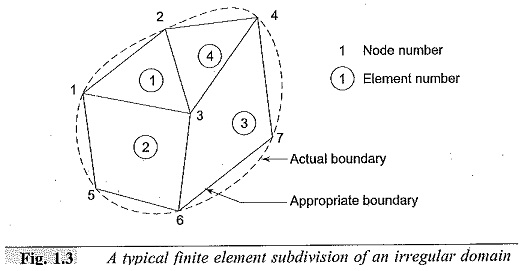
The potential Ve in general is not zero within the element e but it is zero outside the element in view of the fact that the quadrilateral elements are non-confirming elements (see Fig. 1.3).
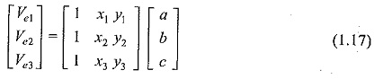
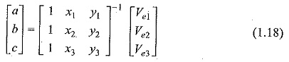
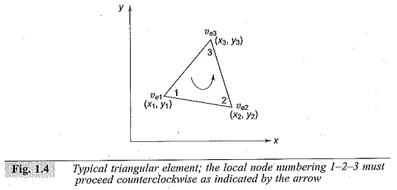
Consider a typical triangular element shown in Fig. 1.4. The potentials Ve1,Ve2 and Ve3 at nodes 1, 2, and 3 are obtained from Eq. (1.15), as
the coefficients a, b, and c are determined from the above equation as
Substituting this equation in Eq. (1.15), we get
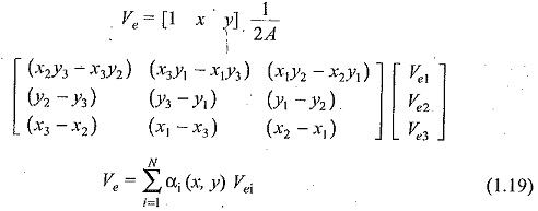
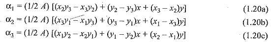
Where,
and A is the area of the element e, that is,
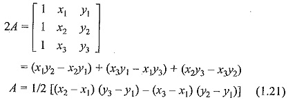
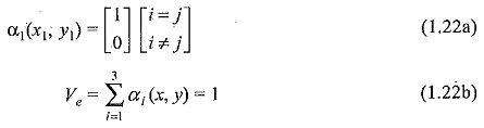
The value of A is positive if the nodes are numbered counterclockwise (starting from any node) as shown by the arrow in Fig. 1.4. It may be noted that Eq. (1.19) gives the potential at any point (x, y) within the element provided that the potentials at the vertices are known. These are called the element shape functions. They have the following properties:
The energy per unit length associated with the element e is given by the following equation:
![]()
where, T denotes the transpose of the matrix
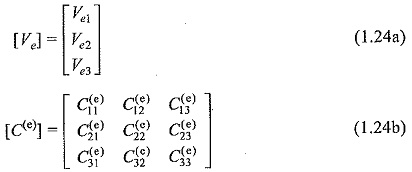
The matrix given above is normally called as element coefficient matrix: The matrix element Cij(e) of the coefficient matrix is considered as the coupling between nodes i and j
(c) Assembling of All Elements
Having considered a typical element, the next stage is to assemble all such elements in the solution region. The energy associated with all the elements will then be
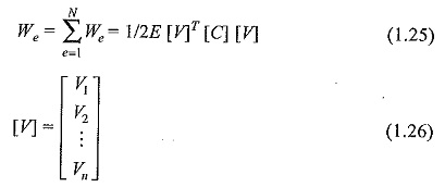
and, n is the number of nodes, N is number of elements and [C] is called the global coefficient matrix which is the sum of the individual coefficient matrices.
(d) Solving the Resulting Equations
It can be shown that the Laplace’s (and Poisson’s) equation is satisfied when the total energy in the solution region is minimum. Thus, we require that the partial derivatives of W with respect to each nodal value of the potential is zero, i.e.
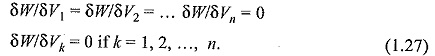
In general, δW/δVk=0 leads to
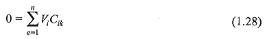
where, n is the number of nodes in the mesh. By writing the above Eq. (1.28) for all the nodes, k = 1, 2, … n, we obtain a set of simultaneous equations from which the solution for V1, V2 … Vn can be found. This can be done either by using the Iteration Method or the Band Matrix Method.
Now, for solving the nodal unknowns, one cannot resort directly to the governing partial differential equations, as a piece-wise approximation has been made to the unknown potential. Therefore, alternative approaches have to be sought. One such classical approach is the calculus of variation. This approach is based on the fact that potential will distribute in the domain such that the associated energy will reach extreme values. Based on this approach, Euler has showed that the potential function that satisfies the above criteria will be the solution of corresponding governing equation. In FEM, with the approximated potential function, extremization of the energy function is sought with respect to each of the unknown nodal potential. This process leads to a set of linear algebraic equations. In this matrix form, these equations form normally a symmetric sparse matrix, which is then solved for the nodal potentials.
Within the individual elements the unknown potential function is approximated by the shape functions of lower order depending on the type of element. An approximate solution of the exact potential is then given in the form of an expression whose terms are the products of the shape function and the unknown nodal potentials. It can be shown that the solution of the differential equation describing the problem corresponds to minimization of the field energy. This leads to a system of algebraic equations the solution for which under the corresponding boundary conditions gives the required nodal potentials. Thus, this procedure results in a potential distribution in the form of discrete potential value at the nodal points of the FEM mesh. The related field strengths at the centres of all elements are then obtained from the potential gradient. The values of the field thus obtained are dependent on the distance between the centres of the elements and the electrode surface, and thus on the sizes of the elements.