Controller Transfer Function:

While a Controller Transfer Function is designed to improve the behavior of a given control system in practice it is very difficult to realize such a controller because of the availability of components. The actual time constant of the controller may deviate from the theoretically designed value. Also the operating conditions may cause a change in plant time constants or even controller time constants. Thus the performance of the system may deviate from the desired or expected one. This incorrect matching may cause differences in the dynamic performance also..

The large time constants of the original system are normally compensated by the time constants of the controller. In other words, the effect of the dominant poles of the plant transfer function is nullified by the zeros of the Controller Transfer Function. This compensation may not be to the desired extent when the actual time constants of the plant vary during operation or the time constants of the controller deviate from the desired ones, for one reason or other.

We shall discuss in the following how the performance of the resulting system gets altered in case of incorrect matching, following a variation in the time constants. We assume that one of the large time constants of the plant varies by a factor K_e leading to the incorrect matching. The transfer function is

which can be written as

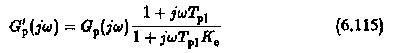
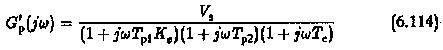
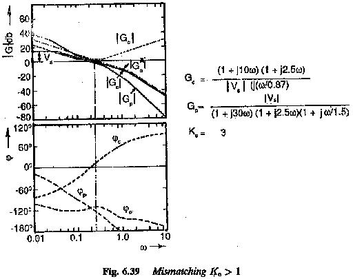
This means that the actual transfer function is the desired transfer function multiplied by a correction factor which is the ratio of (1+jωT_p1)/(1+jωT_p1K_e). The magnitude plot of this ratio depicted in Fig. 6.39. clearly shows that the gain cross-over frequency is above the corner frequency 1/T_p1,1/T_p2. The time response is very much decided by the cross-over frequency. Therefore, the choice of the cross-over frequency plays a significant role in the design of the controller. The frequencies ωT_p1>1 need be considered. In this frequency range the factor 1+jωT_p1/1+jωT_p1 K_e can be simplified as 1/K_e. The transfer function G′_p(jω) simplifies to

The open loop transfer function of the system is

Using the ratio K₀ = T₀/T_e this can be written as

From Eq. 6.117 it can be seen that the ratio K₀ (ratio of integration time of the controller to the uncompensated time constant of the plant) is effectively multiplied by the factor K_e. Thus the change in the time constant is equivalent to a change in this ratio.

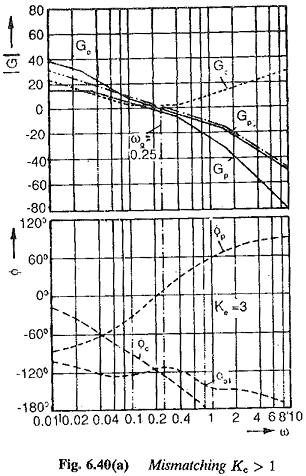
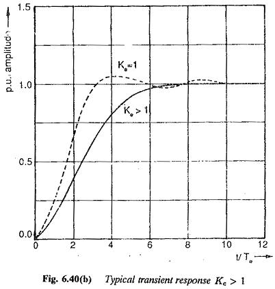
Case (i) K_e > 1 : For this case of K_e > 1, the time constant of the plant increases by this factor. This is equivalent to increase in the ratio K₀ to value K′₀ = K₀K_e. This is equivalent to increase in the integration of the controller. The Bode plots of the functions of the actual and desired transfer functions are shown in Fig. 6.40(a). From the Bode Plots the effects of increase in the time constants can be observed to be the following:

1. Following an increase in the K₀ the Bode plot moves to the left. This results in smaller values of gain cross-over frequency.
2. The phase of the system at the gain cross-over decreases and hence phase margin increases.

3. The value of K₀ as well as the phase margin are related to damping of the system. Increased phase margin results in an increased damping or directly damping = √K′₀/2.
4. Peak overshoot decreases. Some times an overdamped system may also

A typical time response of the resulting second order system for K_e > 1 is shown in Fig, 6.40(b). For comparison the time response for K_e = 1, is also shown in the figure.

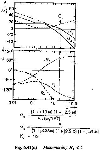
Case (ii) K_e < 1: For this case of K_e < 1 the time constant of the plant decreases by the factor K_e. In this case the situation is different and it is equivalent to decrease in K₀ and hence in the integration time of the Controller Transfer Function. The effect of this on Bode plots shown in Fig. 6.41(a) can be seen to be the following:

1. The amplitude plots of frequency response move towards the right following a decrease in K₀. The gain cross-over for this case occurs at higher The gain cross-over frequency increases.
2. The phase of the transfer function at gain cross-over increases. The phase margin, therefore, decreases.
3. The damping of the system decreases, resulting in an oscillatory response.
4. The peak overshoot is greater than that of the desired one.

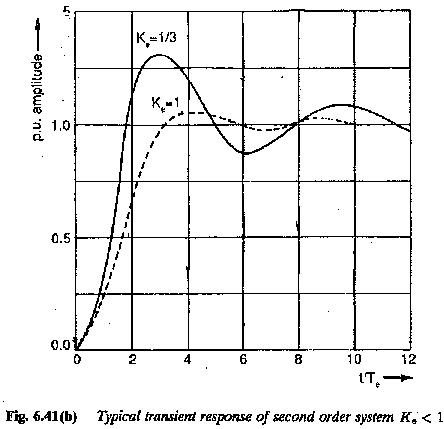
A typical time response for this case is depicted in Fig. 6.41(b).

Therefore the system may have its damping increased or decreased, depending upon whether the compensated time constants increase or decrease in the operation, causing an incorrect matching of the plant with the Controller Transfer Function. From the time responses shown in Figs 6.40(b) and 6.41(b) a deviation of K_e in the range 0.5 < K_e < 2.0 can be allowed.

In a similar way the effect of incorrect matching due to variations in the controller time constants can be modified. For this case the Controller Transfer Function due to incorrect matching is

which can be written as

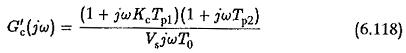
By the same argument that the frequencies of interest are such that ωT_p1≫1 the correction factor (1+jωK_cT_p1)/(1+jωT_p1) can be replaced by K_e. Therefore

The open loop transfer function of the system is

which can be written as

Thus the change in the time constant of the Controller Transfer Function may be studied by an equivalent change in the value of K₀.

A study shows that the effect of reduction in the controller time constant has the same effect as an increase in plant time constant.

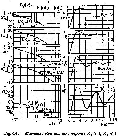
Case (i) K_f < I This case is equivalent to causing an increase in K₀ or increase in the integration time of the Controller Transfer Function. The effects that follow are the same those caused for K_e > 1. The gain cross-over frequency decreases and phase margin increases. The damping (d=√K₀/2) increases. The peak overshoot decreases if the system is still under damped. There is a possibility for the system to become over damped (Fig. 6.42).

Case (ii) K_f > 1: The effect is equivalent to a decrease in the integration time. The effects for the case are the same as those caused for  K_e < 1, viz., the gain cross-over frequency increases, phase margin decreases, the damping decreases causing an increase in peak overshoot. The magnitude plots and time responses are shown in Fig. 6.43 for different values of K₀. These responses confirm the above conclusions. A very low value of K₀ results in a very lightly damped system. Allowable variation K₀ is in the range 1 — 1.5(d = 0.5).

From the above discussion it is clear that the effect of incorrect matching due to increase in the time constants compensated is the same as those due to decrease in the compensating constant of the controller.